Confocor3 two channel cross-correlation

The raw FCS data format of the Zeiss Confocor3 is relatively simple. Zeiss Confocor3 raw files store time-difference between photons. A relatively small header is followed by a set of 32-bit integers that contain the time difference to the previous registered photon. Photons registered by different channels are stored in separate files.

In this example two raw files of a Confocor3 are read and merged into a single photon stream. Next, the merged photon stream is used to compute the cross-correlation between the two channels.

import pathlib
import numpy as np

import pylab as plt
import tttrlib

Reading data

The photon data registered by different detectors are saved in separate files. Read the data of all channels that should be correlated into separate containers.

fns = [str(p) for p in pathlib.Path('../../tttr-data/cz/fcs').glob('5a6ce6a348a08e3da9f7c0ab4ee0ce94_R1_P1_K1_Ch*.raw')]
tttr_data = [tttrlib.TTTR(fn, 'CZ-RAW') for fn in fns]

We combine the data in different files into a single TTTR container using the header of first file as template.

header = tttr_data[0].header
channels = [t.routing_channels[0] for t in tttr_data]
print("Used channels:", channels)

Used channels: [1, 2]

You can check the count rates of the channels using the macro time resolution contained in the header

macro_time_resolution = header.macro_time_resolution
count_rates = [len(t) / (t.macro_times[-1] * macro_time_resolution) for t in tttr_data]
print("Count rates:", count_rates)

Count rates: [148447.28686534363, 183273.524475113]

Now we merge the data of the two detectors in a single container. The marco times need to be sorted first.

macro_times = np.concatenate([t.macro_times for t in tttr_data])
routing_channels = np.concatenate([t.routing_channels for t in tttr_data])
sorted_indices = np.argsort(macro_times)

Using the sorted macro times we sort the routing channel numbers and the macro times.

routing_channels = routing_channels[sorted_indices]
macro_times = macro_times[sorted_indices]

Note: no micro time and no event type in the raw Confocor3 format. Thus, we use ones for the micro time and the event type.

micro_times = np.ones_like(macro_times, dtype=np.uint16)
event_types = np.ones_like(macro_times, dtype=np.int8)

Using the merged marcro times and channel numbers, we create a new TTTR container.

tttr_merged = tttrlib.TTTR()
tttr_merged.set_header(header)
tttr_merged.append_events(
    macro_times=macro_times,
    micro_times=micro_times,
    routing_channels=routing_channels,
    event_types=event_types
)

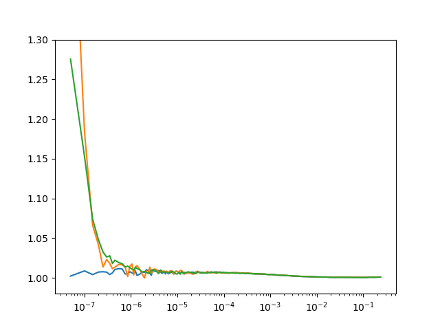
The container can be used for standard analysis, e.g., correlations.

settings = {
    "n_bins": 9,  # n_bins and n_casc defines the settings of the multi-tau
    "n_casc": 19,  # correlation algorithm
}

# Create correlator
# Caution: x-axis in units of macro time counter
# tttrlib.Correlator is unaware of the calibration in the TTTR object
correlator = tttrlib.Correlator(
    channels=([1], [2]),
    tttr=tttr_merged,
    **settings
)
plt.semilogx(
    correlator.x_axis,
    correlator.correlation,
    label="Corr(1,2)"
)

correlator = tttrlib.Correlator(
    channels=([1], [1]),
    tttr=tttr_merged,
    **settings
)
plt.semilogx(
    correlator.x_axis,
    correlator.correlation,
    label="Corr(1,1)"
)

correlator = tttrlib.Correlator(
    channels=([2], [2]),
    tttr=tttr_merged,
    **settings
)
plt.semilogx(
    correlator.x_axis,
    correlator.correlation,
    label="Corr(2,2)"
)

plt.ylim(0.98, 1.30)
plt.show()