Count rate filtered correlation

Overview

The background in the fluorescence intensity affects the computed fluorescence correlation curves. To mitigate the effect of the background on the correlation curves, low count rate regions in a photon stream can be discriminated before correlation.

The example below illustrates a correlation analysis for a single molecule FRET experiments to illustrate different options to discriminate low count rate regions in a photon stream for computing correlation functions of background filtered data.

Note, in the single-molecule example data the background has a significant contribution to the correlation functions. In the example a sliding time-window (TW) is used to select regions in the photon stream with less than a certain amount of photons that are discriminated.

Such a filter can be used to remove the background in a single-molecule experiment that decreased the correlation amplitude.

import numpy as np
import matplotlib.pylab as plt
import tttrlib

Implementation

First, we do a normal correlation where all unfiltered data is correlated. For that, we first read the data into a TTTR container.

data = tttrlib.TTTR('../../tttr-data/bh/bh_spc132.spc', 'SPC-130')

We use a dictionary that contains the most relevant parameters for the correlation algorithm, i.e., the number of bins, n_bins, and the number of coarsening steps, n_casc, as we are going to reuse these parameters later. n_bins and n_casc define the settings of the multi-tau correlation steps. If make_fine is set to false the micro time is not used for correlation.

settings = {
    "n_bins": 3,
    "n_casc": 27,
    "make_fine": False
}

In the TTTR data the channel number 0 and 8 correspond to the green detectors. Here, ([0], [8]) is a correlation of the photons in the channel [0] and the photons in channel [8].

corr_channels_green = ([0], [8])  # green detectors
correlator_green = tttrlib.Correlator(
    tttr=data,
    channels=corr_channels_green,
    **settings
)

Now, we compute the green-red cross correlation. The red detectors correspond to the channel numbers [1,9]. Thus, our input for the correlator is ([0, 8], [1, 9]). This means, that all photons in the green channels [0, 8] are correlated to the photons in the channel [1, 9].

channels_green_red = ([8, 0], [1, 9])
correlator_green_red = tttrlib.Correlator(
    tttr=data,
    channels=channels_green_red,
    **settings
)

To reduce the contribution of scattered light on the correlation we select regions in the TTTR stream that have a minimum count rate. Here, we select regions with at least 60 photons in time windows of 10 ms. Part of the photon stream is selected either by creating a list of indices that refer to TTTR events. These indices are used to create a new TTTR object by slicing the original TTTR object. Below two options to create such a selection is illustrated.

filter_options = {
    'n_ph_max': 60,
    'time_window': 10.0e-3,  # = 10 ms (macro_time_resolution is in seconds)
    'invert': True  # set invert to True to select TW with more than 60 ph
}

A selection can be made using the function selection_by_count_rate or using the method get_selection_by_count_rate. Alternatively, a new TTTR object can be created directly using the filter options and the get_tttr_by_count_rate method of a TTTR object.

selection_idx = tttrlib.selection_by_count_rate(
        time=data.macro_times,
        macro_time_calibration=data.header.macro_time_resolution,
        **filter_options
    )
selection_idx = data.get_selection_by_count_rate(**filter_options)
tttr_selection = data[selection_idx]
tttr_selection = data.get_tttr_by_count_rate(**filter_options)

Next, we computed correlations for the green/green and green/red.

correlator_green_filtered = tttrlib.Correlator(
    channels=corr_channels_green,
    tttr=tttr_selection,
    **settings
)
correlator_green_red_filtered = tttrlib.Correlator(
    channels=channels_green_red,
    tttr=tttr_selection,
    **settings
)

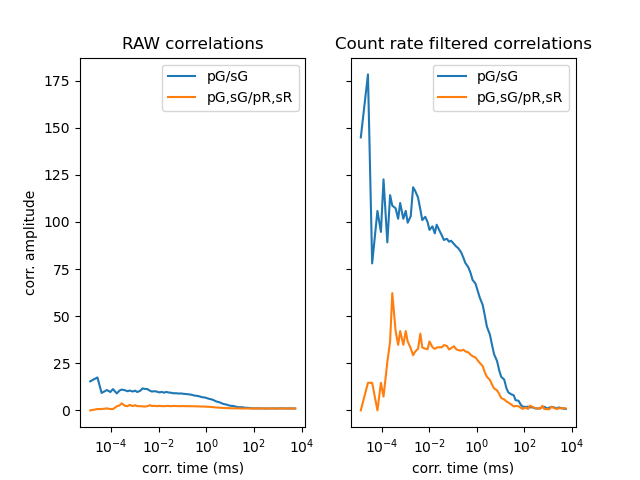
The correlation amplitudes of the correlation curves for data with discriminated background is considerably higher as seen in the plots of the raw and unfiltered correlations.

fig1, ax = plt.subplots(1, 2, sharex='col', sharey='row')
ax[0].semilogx(
    correlator_green.x_axis * 1000.0,
    correlator_green.correlation,
    label="pG/sG"
)
ax[0].set_xlabel('corr. time (ms)')
ax[0].set_ylabel('corr. amplitude')
ax[0].semilogx(
    correlator_green_red.x_axis * 1000.0,
    correlator_green_red.correlation,
    label="pG,sG/pR,sR"
)
ax[0].set_title('RAW correlations')
ax[0].legend()
ax[1].semilogx(
    correlator_green_filtered.x_axis * 1000.0,
    correlator_green_filtered.correlation,
    label="pG/sG"
)
ax[1].set_xlabel('corr. time (ms)')
ax[1].semilogx(
    correlator_green_red_filtered.x_axis * 1000.0,
    correlator_green_red_filtered.correlation,
    label="pG,sG/pR,sR"
)
ax[1].legend()
ax[1].set_title('Count rate filtered correlations')
plt.show()

Count rate threshold

The threshold for the count rate filter has an effect on the computed correlation functions. To illustrate the effect of the count rate filter on the correlation amplitude we will vary the threshold value for the filter and compute correlation functions for each filter value. To decrease the computation time, we decrease the number of bins in a correlation curve. For reference, we compute the correlation curve of the unfiltered data.

corr_settings = {
    "n_bins": 2,
    "n_casc": 30
}
correlator = tttrlib.Correlator(tttr=data, channels=corr_channels_green, **corr_settings)
x_unfiltered, y_unfiltered = correlator.x_axis, correlator.correlation

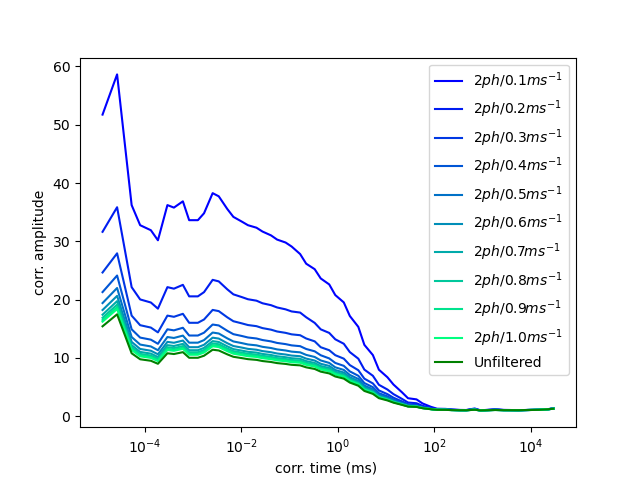
Next, we define the filter parameter values. Here, we select for time windows (TWs) with at least two photons in time windows of 10 seconds.

n_ph = 2
filter_options = {
    'n_ph_max': n_ph,
    'time_window': 10.0,  # 10 seconds
    'invert': True  # set invert to True to select TW with more than 50 ph
}

Using our values defines for the filter, we repeat the correlation calculations several times for different time windows. Here, we vary the time window from 0.1 ms to 1 ms and require that each time window has at least two photons.

correlations = list()
n_tw = 10
tws = np.linspace(1e-4, 1e-3, n_tw)
for tw in tws:
    filter_options['time_window'] = tw
    tttr = data.get_tttr_by_count_rate(**filter_options)
    correlator = tttrlib.Correlator(tttr=tttr, **corr_settings, channels=corr_channels_green)
    correlations.append(correlator.correlation)
correlations = np.array(correlations)

Finally, we plot the resulting correlation curves. As expected, the correlation amplitude of correlation curves computed for smaller TWs (higher count rate) is higher. Note, this effect can be used in methods such as Photon Arrival-Time Interval Distribution (PAID) to resolve species mixtures [laurence2004].

# Plot the raw/unfiltered correlations
fig2, ax = plt.subplots(nrows=1, ncols=1)
ax = [ax]
labels = [r"$%s ph / %.1f ms^{-1}$" % (n_ph, x * 1000) for x in tws]
colormap = plt.cm.winter
ax[0].set_prop_cycle(plt.cycler('color', colormap(np.linspace(0, 1, n_tw))))
for i, corr in enumerate(correlations):
    ax[0].semilogx(x_unfiltered * 1000.0, corr, label=labels[i])
ax[0].semilogx(x_unfiltered * 1000.0, y_unfiltered, color="green", label="Unfiltered")
ax[0].legend()
ax[0].set_xlabel(r'corr. time (ms) ')
ax[0].set_ylabel(r'corr. amplitude')
plt.show()