Estimating the noise of the correlation curves

Introduction

There are many approaches to estimate the noise in correlation functions (see: [Wohland2001], [Qian1990], [Starchev2001]). An analytical calculation of the noise is difficult because it involves diverging integrals for the correlations decaying functions [Wohland2001]. For TTTR data an analytical solution of the noise in the correlation is however not necessary, as the data contained in the photon stream can be split to yield a set of correlation functions that is used to yield an estimate for the expected correlation function and the associated noise by the mean and the standard deviation [Kapusta2007], [Enderlein1997], [Bohmer2002].

Here it is illustrated how the data is split into multiple subsets to estimate the noise for quantitative analysis of correlation curves.

Implementation

First, we import libraries read the data into a new TTTR container. We inspect the header information to find header tags that inform on the macro time calibration.

import pylab as plt
import tttrlib
import numpy as np

data = tttrlib.TTTR('../../tttr-data/pq/ptu/pq_ptu_hh_t2.ptu')

Here, we manually compute the calibration. This may not be necessary in many cases.

time_calibration = data.header.tag('MeasDesc_GlobalResolution')['value']

Next, we split the TTTR data into n_chunks subsets of equal size.

n_chunks = 4
n_ph = int(len(data) / n_chunks)

Before correlating the data, we define the number of bins and the number of coarsening steps for the multi-tau correlation algorithm and create a new correlator instance.

print("Used routing channels:", data.used_routing_channels)
ch1 = [0]
ch2 = [2]
corr_settings = {
    "n_bins": 5,
    "n_casc": 30
}
correlator = tttrlib.Correlator(**corr_settings)

# use start-stop to create new TTTR objects that are correlated
correlations = list()
for i in range(0, len(data), n_ph):
    tttr_slice = data[i: i + n_ph]
    tttr_ch1 = tttr_slice[tttr_slice.get_selection_by_channel(ch1)]
    tttr_ch2 = tttr_slice[tttr_slice.get_selection_by_channel(ch2)]
    correlator.set_tttr(
        tttr_1=tttr_ch1,
        tttr_2=tttr_ch2
    )
    correlations.append(correlator.correlation)
correlations = np.array(correlations)

Used routing channels: [0 2]

Finally, Plot the all correlations plot the unsliced correlation

correlator = tttrlib.Correlator(
    tttr=data,
    channels=(ch1, ch2),
    **corr_settings
)

means = correlations.mean(axis=0)
stds = correlations.std(axis=0)
x_axis = correlator.x_axis
fig, ax = plt.subplots(nrows=1, ncols=2, sharey=True, sharex=True)
ax[0].semilogx(x_axis, correlator.correlation, label="All photons", color="green")
ax[0].semilogx(x_axis, means, label="Mean", color="blue")
ax[0].fill_between(x_axis, means-stds, means+stds, alpha=.5)
ax[0].set_title('Correlation all data')
ax[1].set_title('Correlation of slices')
for y in correlations:
    ax[1].semilogx(x_axis, y)
ax[0].set_ylim([0.9, 3.5])
ax[0].set_xlabel(r'corr. time (s) ')
ax[1].set_xlabel(r'corr. time (s) ')
ax[0].set_ylabel(r'corr. amplitude')
ax[0].legend()
plt.show()

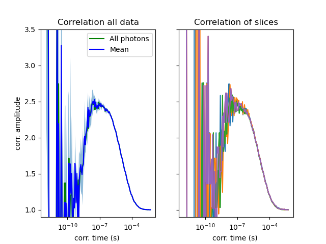
The standard deviation computed over multiple correlation curves can be used as an estimate for the noise.