Full correlation

When processes faster than the macro time clock are of interest, the micro time and the macro time can be combined into a united time axis. Using the combined time axis of a so called full correlation can be performed in continuous wave excitation experiments in contrast to the usually performed pulsed excitation.

The example below illustrates how a full correlation can be computed. Note, in the example the full correlation is computed for a sample that was measured in a pulsed excitation experiment. However, the same procedure can be applied to cw data.

This example illustrates a normal correlation and demonstrates two approaches how to compute full correlations with tttrlib.

import tttrlib
import matplotlib.pylab as plt
import numpy as np

First, we read a dataset into a TTTR container. In the example, we use a small part of a single-molecule multiparameter fluorescence detection experiment with parallel and perpendicular green and red detection channels. We use a small dataset due to practical reasons to illustrate methods how to correlate fluorescence data in tttrlib. For productive analysis of a real experiment usually more data would be processed.

data = tttrlib.TTTR('../../tttr-data/bh/bh_spc132.spc', 'SPC-130')

After reading the data, we create two new TTTR containers for the two correlation channels. Here, we cross-correlate photons in the channels (8, 1) to (0, 9). There are two options how to create TTTR objects for the channels. A new TTTR object can be created with an existing object by providing a list of indices.

ch1_indices = data.get_selection_by_channel([8, 1])
tttr_ch1 = tttrlib.TTTR(data, ch1_indices)

Alternatively, there is a method that creates new TTTR objects for a list of channels:

tttr_ch2 = data.get_tttr_by_channel([0, 9])

The two TTTR objects can be directly cross-correlated. Here, by default the micro times are not considered in the correlation.

correlator_ref = tttrlib.Correlator(
    tttr=(tttr_ch1, tttr_ch2),
    n_casc=25,
    n_bins=7
)
x_normal = correlator_ref.x_axis
y_normal = correlator_ref.correlation

To compute a full correlation, i.e., a correlation that uses the micro times as time information, the default value of parameters make_fine when creating a new Correlator needs to by modified:

full_corr_settings = {
    "n_casc": 37,  # n_bins and n_casc defines the settings of the multi-tau
    "n_bins": 7,  # correlation algorithm
    "make_fine": True  # Use the microtime information (also called "fine" correlation)
}
correlator = tttrlib.Correlator(
    **full_corr_settings,
    tttr=(tttr_ch1, tttr_ch2),
)
x_corr = correlator.x_axis
y_corr = correlator.correlation

In case there is need for a finer control the input for the correlator can be computed manually by first obtaining the macro times, the micro times, computing weights for the photons and setting the macro times, the weights and the micro times manually before obtaining a correlation curve from the correlator.

correlator_ref = tttrlib.Correlator(**full_corr_settings)  # read the settings from above
t1, t2 = data.macro_times[ch1_indices], tttr_ch2.macro_times  # Get the macrotime information
mt1, mt2 = data.micro_times[ch1_indices], tttr_ch2.micro_times  # Get the microtime information
w1, w2 = np.ones_like(t1, dtype=np.float64), np.ones_like(t2, dtype=np.float64)  # Generate weights
# Note: the weights are all set to 1 here, i.e. no weighting
correlator_ref.set_macrotimes(t1, t2)
correlator_ref.set_weights(w1, w2)
n_microtime_channels = data.get_number_of_micro_time_channels()
correlator_ref.set_microtimes(mt1, mt2, n_microtime_channels)
x_ref = correlator_ref.x_axis
y_ref = correlator_ref.correlation
# x-axis needs to be multiplied with microtime resolution to obtain correct timing:
x_ref *= data.header.micro_time_resolution

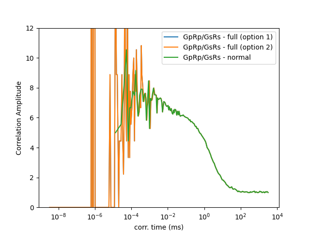
When the macro and the micro times are combined, the correlation curves can be computed for shorter correlation times as illustrated below.

fig, ax = plt.subplots(1, 1, sharex='col', sharey='row')
ax.semilogx(x_corr * 1000, y_corr, label="GpRp/GsRs - full (option 1)")
ax.semilogx(x_ref * 1000, y_ref, label="GpRp/GsRs - full (option 2)")
ax.semilogx(x_normal * 1000, y_normal, label="GpRp/GsRs - normal")
ax.set_xlabel('corr. time (ms)')
ax.set_ylabel('Correlation Amplitude')
ax.legend()
ax.set_ylim(0, 12)  # Set y-axis range to 0-12

plt.show()