Micro time gated correlation

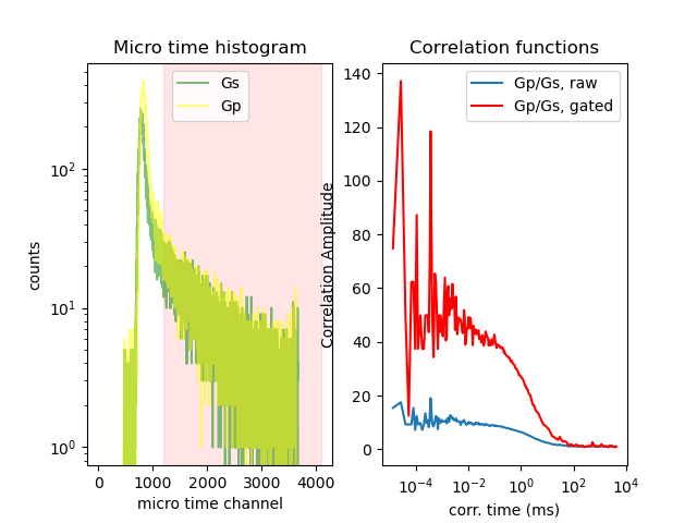
The background in the fluorescence intensity traces affects the computed fluorescence correlation functions. In single-molecule spectroscopy the background is mainly caused by scattered light. Thus, by discriminating photons with small micro times a large fraction of the background can be eliminated.

Note, the example that used the micro times of the detected photons to gate away the scattered light fraction in a single-molecule experiment can be easily modified to correlate the prompt and the delayed excitation in a pulsed interleaved excitation experiment.

import matplotlib.pylab as plt
import tttrlib
import numpy as np

First, the TTTR data is read into a new container. The TTTR data in the example is a multiparameter fluorescence detection data with two green and two red detectors for polarization resolved fluorescence detection.

data = tttrlib.TTTR('../../tttr-data/bh/bh_spc132.spc', 'SPC-130')

Here, we compute the cross correlation function between the parallel (P) and the perpendicular (S) green detection channels. We first find the indices of the respective channels. In the example the channel numbers of the green parallel and perpendicular detection are 0 and 8.

ch1_indices = data.get_selection_by_channel([0])
ch2_indices = data.get_selection_by_channel([8])

For illustrating the scattered light, we create histogram of micro times and define a lower bound to mask photons. Here, n_lower is set based on the micro time histograms, i.e. only bins with significant amount of fluorescence photons are used.

n_micro = data.header.number_of_micro_time_channels
x_hist = np.arange(n_micro)
y_hist_0 = np.bincount(data.micro_times[ch1_indices], minlength=n_micro)
y_hist_8 = np.bincount(data.micro_times[ch2_indices], minlength=n_micro)
n_lower = 1200  # n_lower will be used below in the actual correlation calculation

Next, we create a new correlator and set the numbers of bin and correlation cascades of the multi-tau correlation algorithm. The parameters B and n_casc are the number of correlation channels and the number of coarsening steps. For each coarsening step B correlation amplitudes are computed. Setting these parameters is optional. If they are not defined a set of default parameters is used.

correlator = tttrlib.Correlator()
B = 9
n_casc = 25
correlator.n_bins = B
correlator.n_casc = n_casc

The correlator contains a correlation curve that is updated when the correlator content is marked as invalid, e.g., when the inputs are changed. The curve has a settings (CorrelatorSettings class) attribute that stores the time resolution (used to calibrate the correlation curve). Here, we use a more “manual” approach to compute correlations. Hence, we provide the resolution by hand. In most cases, the resolution is read from the TTTR container.

correlator.curve.settings.macro_time_duration = data.header.macro_time_resolution

Next, we assign the macro times to the correlator with their respective weights. In a normal correlation all photons have equal weights. We get the macrotimes and set the weights, the weights will = 1, i.e. no weighting will be used

t = data.macro_times
t1 = t[ch1_indices]
w1 = np.ones_like(t1, dtype=np.float64)
t2 = t[ch2_indices]
w2 = np.ones_like(t2, dtype=np.float64)
correlator.set_events(t1, w1, t2, w2)

x_raw = correlator.x_axis
y_raw = correlator.correlation

Now, we compute a correlation function where we want to discriminate photons that have a small micro time. For that, we set the weight of photons with a micro time is smaller than n_lower to zero.

t = data.get_macro_times()
mt = data.get_micro_times()
t1 = t[ch1_indices]
mt1 = mt[ch1_indices]
w1 = np.ones_like(t1, dtype=np.float64)
w1[np.where(mt1 < n_lower)] *= 0.0

Mask also the data for ch2 using the microtime information. We mask values by setting the weights where the micro time is smaller than 1500 to zero and masks the photons, i.e. this corresponds to only taking the green photon emitted in the “delay” tine window of the PIE experiment into account for the correlation

t2 = t[ch2_indices]
mt2 = mt[ch2_indices]
w2 = np.ones_like(t2, dtype=np.float64)
w2[np.where(mt2 < n_lower)] *= 0.0

correlator.set_events(t1, w1, t2, w2)
x_gated = correlator.x_axis
y_gated = correlator.correlation

The correlation amplitude of the correlation curve computed for all photons is lower than the correlation amplitude computed for photons with a larger micro time.

fig, ax = plt.subplots(1, 2)
ax[0].set_title('Micro time histogram')
ax[0].axvspan(n_lower, n_micro, color='red', alpha=0.1)
ax[0].semilogy(x_hist, y_hist_0, label="Gs", color="green", alpha=0.5)
ax[0].semilogy(x_hist, y_hist_8, label="Gp", color="yellow", alpha=0.5)
ax[0].set_xlabel('micro time channel')
ax[0].set_ylabel('counts')
ax[0].legend()
ax[1].semilogx(x_raw * 1000, y_raw, label="Gp/Gs, raw")
ax[1].set_title('RAW correlations')
ax[1].set_xlabel('corr. time (ms)')
ax[1].set_ylabel('Correlation Amplitude')
ax[1].semilogx(x_gated * 1000, y_gated, label="Gp/Gs, gated", color='red')
ax[1].set_xlabel('corr. time (ms)')
ax[1].set_title('Correlation functions')
ax[1].legend()
plt.show()