Normal multi-tau correlation

An alternative approach is to calculate the FCS curve by software on the basis of the directly recorded asynchronous photon count data. The straightforward approach would be to generate a continuous file of fluorescence intensity values in consecutive time bins of fixed bin width, and to use this file for a conventional autocorrelation calculation. But then again, one encounters the same unreasonably large amount of data as when directly recording fluorescence intensity values in a synchronous data acquisition mode.

When applying the algorithm only at the increasingly spaced lag times as given by Eq. (2), it will completely miss, e.g., the strong autocorrelation of any periodic signal with a repetition time not included within the vector of used lag times. To avoid that, one usually applies an averaging procedure by coarsening the time resolution of the photon detection times tj when coming to the calculation of the autocorrelation function at increasingly larger lag time. This is equivalent to the multiple-tau and multiple-sampling time correlation method employed in hardware correlators [12].

[Wahl2003].

import matplotlib.pylab as plt
import tttrlib
import numpy as np


fig, ax = plt.subplots(sharex='col', sharey='row')

#  Read the data data
data = tttrlib.TTTR('../../tttr-data/bh/bh_spc132.spc', 'SPC-130')

# Correlator settings, if the same settings are used repeatedly it is useful to define them once
settings = {
    "n_bins": 7,  # n_bins and n_casc defines the settings of the multi-tau
    "n_casc": 27,  # correlation algorithm
    "make_fine": False  # Do not use the microtime information
}

# Create correlator
# Caution: x-axis in units of macro time counter
# tttrlib.Correlator is unaware of the calibration in the TTTR object
correlator = tttrlib.Correlator(**settings)

# Select the green channels (channel number 0 and 8)
ch1_indices = data.get_selection_by_channel([0])
ch2_indices = data.get_selection_by_channel([8])

# Select macro times for Ch1 and Ch2 and create array of weights
# Note: the weights are set to 1, i.e. no weighting is used
t = data.macro_times
t1 = t[ch1_indices]
w1 = np.ones_like(t1, dtype=np.float64)
t2 = t[ch2_indices]
w2 = np.ones_like(t2, dtype=np.float64)
correlator.set_events(t1, w1, t2, w2)

# scale the x-axis to have units in milliseconds (common unit in FCS)
x = correlator.x * data.header.macro_time_resolution
y = correlator.y

plt.semilogx(x, y, label="Gp/Gs")

# green-red cross correlation (red channels 1 and 9)
# TODO: verify "if the correlator is generated using the architecture below,
# the macro time units are known and no rescaling of the y-axis needs to be performed"
correlator = tttrlib.Correlator(
    tttr=(
        tttrlib.TTTR(data, data.get_selection_by_channel([0, 8])),
        tttrlib.TTTR(data, data.get_selection_by_channel([1, 9]))
    ),
    **settings
)

# no need to scale axis - correlator aware of macro time units
plt.semilogx(
    correlator.x,
    correlator.y,
    label="Gp,Gs/Rp,Rs"
)

# red channel correlation
correlator = tttrlib.Correlator(
    channels=([9], [1]),
    tttr=data,
    **settings
)

plt.semilogx(
    correlator.x,
    correlator.y,
    label="pR,sR"
)

# Reverse cross-correlation: red-green
correlator = tttrlib.Correlator(
    channels=([9, 1], [0, 8]),
    tttr=data,
    **settings
)

plt.semilogx(
    correlator.x,
    correlator.y,
    label="pRsR,pGsG"
)

# Show results
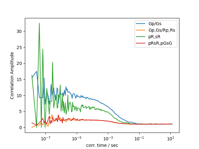
plt.xlabel('corr. time / sec')
plt.ylabel('Correlation Amplitude')
plt.legend()

plt.show()