FLIM-PIE

In Pulsed interleaved excitation (PIE) the sample is excited by more than one light source. The exciting light source is usually a pulsed laser. When analyzing the detected fluorescence the interleaved excitation needs to be taken into account. For that, when two excitation sources are used, the micro time detection windows is separted into two ranges, a prompt range (a blue laser excites the donor in a FRET experiment) and the delay range (a red laser excites the acceptor in a FRET experiment).

Import all required libraries

import tttrlib
import numpy as np
import matplotlib.pyplot as plt
import skimage as ski
import skimage.filters
import skimage.morphology
import skimage.util
import scipy
import scipy.ndimage


def plot_images(images, titles, cmaps=None, **kwargs):
    if cmaps is None:
        cmaps = ['viridis'] * len(images)
    if titles is None:
        titles = [''] * len(images)
    fig, ax = plt.subplots(**kwargs)
    ax = ax.flatten()
    for i, img in enumerate(images):
        im = ax[i].imshow(img, cmap=cmaps[i])
        ax[i].set_title(titles[i])
        fig.colorbar(im, ax=ax[i], fraction=0.046, pad=0.04)
    return fig, ax

Loading data

First, we read the TTTR data, create CLSM image container, and define used channels. We create a CLSM container for the green photons and the red photons. Moreover, we create containers for red photons in the prompt and the delay time window.

filename_data = '../../tttr-data/imaging/pq/ht3/mGBP_DA.ht3'
tttr_data = tttrlib.TTTR(filename_data)

clsm_green = tttrlib.CLSMImage(tttr_data)
clsm_red = tttrlib.CLSMImage(tttr_data)
clsm_red_prompt = tttrlib.CLSMImage(tttr_data)
clsm_red_delay = tttrlib.CLSMImage(tttr_data)

green_ch = [0, 1]
red_ch = [4, 5]
sum_all = green_ch + red_ch

Define PIE windows

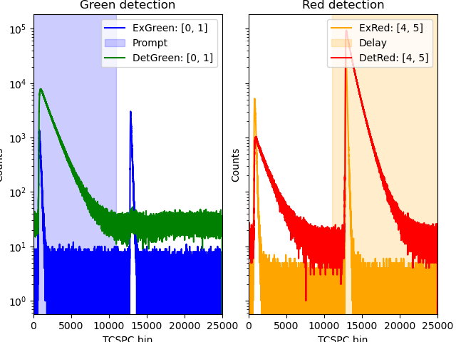
In PIE two light sources excite the sample. Here, we load the instrument response function (IRF) and inspect the IRFs of the two separate the fluorescence of the first (prompt) and the second (delay) excitation pulse. The two excitation pulses define two micro time detection windows for the prompt and the delay pulse.

filename_irf = '../../tttr-data/imaging/pq/ht3/mGBP_IRF.ht3'

irf = tttrlib.TTTR(filename_irf)
tttr_irf_green = irf.get_tttr_by_channel(green_ch)
tttr_irf_red = irf.get_tttr_by_channel(red_ch)

tttr_green = tttr_data.get_tttr_by_channel(green_ch)
tttr_red = tttr_data.get_tttr_by_channel(red_ch)
microtime_hist_green = tttr_green.microtime_histogram
microtime_hist_red = tttr_red.microtime_histogram

n_micro = tttr_data.header.number_of_micro_time_channels
prompt_range = 0, 11000
delay_range = 11000, 25000
fig, ax = plt.subplots(nrows=1, ncols=2, sharex=True, sharey=True)
fig.tight_layout()
ax[0].semilogy(tttr_irf_green.microtime_histogram[0], label="ExGreen: %s" % green_ch, color="blue")
ax[0].axvspan(*prompt_range, color='blue', alpha=0.2, label="Prompt")
ax[1].semilogy(tttr_irf_red.microtime_histogram[0], label="ExRed: %s" % red_ch, color="orange")
ax[1].axvspan(*delay_range, color='orange', alpha=0.2, label="Delay")
ax[0].semilogy(microtime_hist_green[0], color="green", label="DetGreen: %s" % green_ch)
ax[1].semilogy(microtime_hist_red[0], color="red", label="DetRed: %s" % red_ch)
ax[0].set(xlabel='TCSPC bin', ylabel='Counts', title='Green detection')
ax[1].set(xlabel='TCSPC bin', ylabel='Counts', title='Red detection')
ax[0].legend()
ax[1].legend()
ax[0].set_xlim(0, 25000)
ax[1].set_xlim(0, 25000)
plt.show()

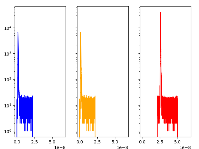
Create a mask to select photons in certain channel and in micro time range to split the photons in prompt and delay.

mask_irf_green_prompt = tttrlib.TTTRMask()
mask_irf_green_prompt.select_channels(irf, green_ch)
mask_irf_green_prompt.select_microtime_ranges(irf, [prompt_range])
tttr_irf_green_prompt = irf[mask_irf_green_prompt.indices]

mask_irf_red_prompt = tttrlib.TTTRMask()
mask_irf_red_prompt.select_channels(irf, red_ch)
mask_irf_red_prompt.select_microtime_ranges(irf, [prompt_range])
tttr_irf_red_prompt = irf[mask_irf_red_prompt.indices]

mask_irf_red_delay = tttrlib.TTTRMask()
mask_irf_red_delay.select_channels(irf, red_ch)
mask_irf_red_delay.select_microtime_ranges(irf, [delay_range])
tttr_irf_red_delay = irf[mask_irf_red_delay.indices]

fig, ax = plt.subplots(nrows=1, ncols=3, sharex=True, sharey=True)
fig.tight_layout()
ax[0].semilogy(*tttr_irf_green_prompt.microtime_histogram[::-1], color='blue')
ax[1].semilogy(*tttr_irf_red_prompt.microtime_histogram[::-1], color='orange')
ax[2].semilogy(*tttr_irf_red_delay.microtime_histogram[::-1], color='red')
fig.show()

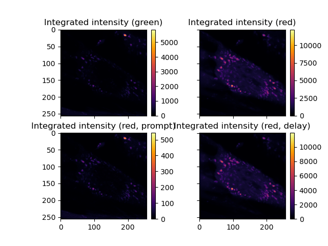
Intensity imaging

Fills the CLSM image container with intensities. The green CLSM container gets filled with all photons (independent of the excitation pulse), as the red laser does not excite the sample.

clsm_green.fill(tttr_data, channels=green_ch)  # green channels

If not specified the red channel includes the photons in the prompt and the delay. Red intensity is total intensity, ie, prompt + delayed excitation

clsm_red.fill(tttr_data, channels=red_ch)

To separate the photons by the micro time specify the micro time range.

clsm_red_prompt.fill(channels=red_ch, micro_time_ranges=[prompt_range])
clsm_red_delay.fill(channels=red_ch, micro_time_ranges=[delay_range])

# An intensity image the number of counts in a pixel corresponds to the number of photons
fig, _ = plot_images(
    [
        clsm_green.intensity.sum(axis=0),
        clsm_red.intensity.sum(axis=0),
        clsm_red_prompt.intensity.sum(axis=0),
        clsm_red_delay.intensity.sum(axis=0)
    ],
    titles=[
        'Integrated intensity (green)',
        'Integrated intensity (red)',
        'Integrated intensity (red, prompt)',
        'Integrated intensity (red, delay)'
    ],
    cmaps=['inferno', 'inferno', 'inferno', 'inferno'],
    nrows=2, ncols=2, sharex=True, sharey=True
)
fig.show()

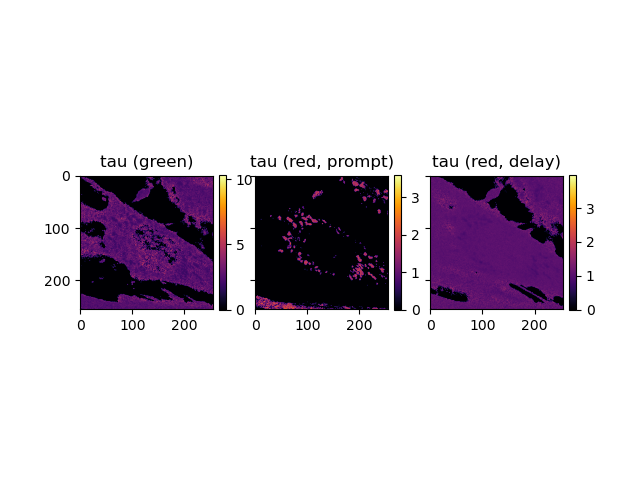
Intensity imaging

settings_lt = {
    "tttr_data": tttr_data,
    "minimum_number_of_photons": 30,
    "stack_frames": True
}
mean_tau_green = clsm_green.get_mean_lifetime(
    tttr_irf=tttr_irf_green_prompt, **settings_lt
)

mean_tau_red_prompt = clsm_red_prompt.get_mean_lifetime(
    tttr_irf=tttr_irf_red_prompt, **settings_lt
)

mean_tau_red_delay = clsm_red_delay.get_mean_lifetime(
    tttr_irf=tttr_irf_red_delay, **settings_lt
)

fig, _ = plot_images(
    [
        mean_tau_green.sum(axis=0),
        mean_tau_red_prompt.sum(axis=0),
        mean_tau_red_delay.sum(axis=0)
    ],
    titles=[
        'tau (green)',
        'tau (red, prompt)',
        'tau (red, delay)'
    ],
    cmaps=['inferno', 'inferno', 'inferno'],
    nrows=1, ncols=3, sharex=True, sharey=True
)
plt.show()