TTTR Image representations

TTTR images are mappings from pixels to groups of photons. The photons relate to a set of pulsed light sources that illuminate the sample. The photons are detected by a set of detectors and the time between the light pulse and the detection is registered along with a detector identifier using time-resolved detection. To visualize features of photon groups that relate to the pixel a dimensionality reduction is applied.

Here, few examples visualize typical mappings from photon groups to representations that can be visualized in an image. In this example data of a pulsed interleaved (PIE) multiparameter fluorescence detection (MFD) Förster Resonance Energy Transfer (FRET) experiment is processed. The FRET sample contained a donor, D, and an acceptor, A, fluorophore. Using the data contained in the TTTR file, we:

1. create intensity images

2. selection of channels

3. stripping of photons from CLSMImage

4. image of the mean micro times

5. a fluorescence intensity decay of the micro times

#%
from __future__ import print_function

import matplotlib.pyplot as plt
import numpy as np
import pylab as p
import tttrlib


def plot_images(images, titles, cmaps=None, **kwargs):
    if cmaps is None:
        cmaps = ['viridis'] * len(images)
    if titles is None:
        titles = [''] * len(images)
    fig, ax = plt.subplots(**kwargs)
    ax = ax.flatten()
    for i, img in enumerate(images):
        im = ax[i].imshow(img, cmap=cmaps[i])
        ax[i].set_title(titles[i])
        fig.colorbar(im, ax=ax[i], fraction=0.046, pad=0.04)
    return fig, ax

The FLIM dataset consists of a measurement of the sample and an instrument response function (IRF). We inspect the used routing channels to make sure which detectors have been used in the measurement.

data = tttrlib.TTTR('../../tttr-data/imaging/pq/ht3/mGBP_DA.ht3')
irf = tttrlib.TTTR('../../tttr-data/imaging/pq/ht3/mGBP_IRF.ht3')
print("Used routing channels: ", data.used_routing_channels)

#%
# Next, we define lists over routing channel numbers that we
# will use later to refer to different detectors. Here, we
# are going to inspect the routing channel number 0, and 1,
# that correspond for the dataset of the experiment to the
# parallel (P) and perpendicular detector (S). We plan to make
# FLIM images for P, S, and P+S combined.
detection_channels = {
    "Gps": {  # Green total
        "channels": [0, 1]
    },
    "Gp": {  # Green parallel
        "channels": [0]
    },
    "Gs": {  # Green perpendicular
        "channels": [1]
    },
    "Rps": {  # Green total
        "channels": [4, 5]
    },
    "Rp": {  # Green parallel
        "channels": [4]
    },
    "Rs": {  # Green perpendicular
        "channels": [5]
    }
}

Used routing channels:  [4 5 0 1 2]

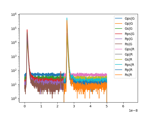
The FLIM dataset is a Pulsed-Interleaved-Excitation (PIE) dataset. In PIE experiments, the sample is sequentially excited by light sources of different wavelength. In our dataset the sample is first excited by a laser that predominantly excites the donor. Here we define a range of micro time channels that we are using to define a “Prompt” and a “Delay”. The prompt microtime range captures the fluorescence, F, of the green, F(G|G), and red, F(R|G), detectors, given the green excitation light source, G. The delay microtime channels capture the fluorescence given an excitation by the red, R, light source (F(R|R), F(G|R)). In the data acquired in an MFIS (Multiparameter Fluorescence Image spectroscopy) the green and red fluorescence is moreover split into P and S. Here, we will only inspect data in F(G|G) and F(R|G).

excitation_windows = {
    "G": {  # Green excitation
        "micro_time_ranges": [(0, 12000)]
    },
    "R": {  # Red excitation
        "micro_time_ranges": [(12000, 32000)]
    }
}

#%
# Here we create all combinations of excitation and detection
# channels. For the example: G|G, G|R, R|G, R|R
fill_settings = {}
for ex in excitation_windows:
    d = dict()
    for ch in detection_channels:
        d[ch] = {}
        d[ch].update(detection_channels[ch])
        d[ch].update(excitation_windows[ex])
    fill_settings[ex] = d

#%
# Create a dictionary that contains the IRF photons
# for the respective Det|Exc pairs
irfs = dict()
for ex in excitation_windows:
    irfs[ex] = dict()
    for ch in detection_channels:
        microtime_range = fill_settings[ex][ch]['micro_time_ranges']
        chs = fill_settings[ex][ch]['channels']
        irf_mt_idx = np.where(
            (irf.micro_times > microtime_range[0][0]) &
            (irf.micro_times < microtime_range[0][1])
        )[0]
        irf_ch_idx = irf.get_selection_by_channel(chs)
        irf_idx = np.intersect1d(irf_mt_idx, irf_ch_idx)
        irf_sel = irf[irf_idx]
        irfs[ex][ch] = irf_sel

Next, we plot the IRFs for the different combinations of excitation pulses and detectors.

for ex in irfs:
    name_ex = "%s" % ex
    for det in irfs[ex]:
        name_det = "%s" % det
        name = name_det + "|" + name_ex
        irf_x = irfs[ex][det]
        plt.semilogy(
            *irf_x.get_microtime_histogram(micro_time_coarsening=16)[::-1],
            label=name
        )
plt.legend()
plt.show()

Create image

image = tttrlib.CLSMImage(data)

In case an automated processing of header does not wor reads header but does not always work, frame marker, line marker, etc. more details (in case it does not work without providing markers)

clsm_settings = {
    "marker_frame_start": [4],
    "marker_line_start": 1,
    "marker_line_stop": 2,
    "marker_event_type": 1,
    "n_pixel_per_line": 256,
    "reading_routine": 'default',
    "skip_before_first_frame_marker": True
}

image = tttrlib.CLSMImage(data, **clsm_settings)

#%
# Here, we only look at the green photons (simplicity)
image.fill(**fill_settings["G"]["Gps"])
print("Fill settings:%s" % fill_settings["G"]["Gps"])

#%
# Intensity images
# ----------------
# Frames, lines, pixel
image_intensity_green = image.intensity
# this is equivalent to
image_intensity_green = image.get_intensity()
image_intensity_green_sum = image_intensity_green.sum(axis=0)

Fill settings:{'channels': [0, 1], 'micro_time_ranges': [(0, 12000)]}

Plot images Intensity images

plot_images(
    images=[
        image_intensity_green[30],
        image_intensity_green.sum(axis=0)
    ],
    titles=[
        'Intensity of a single frame ch:%s' % detection_channels['Gps'],
        'Intensity of integrated frames ch:%s' % detection_channels['Gps']
    ],
    ncols=2, nrows=1
)


#%
# Micro time  images
# ------------------
# 1. Mean micro time
# 2. Mean lifetime
# 3. Histogram over micro times
#
minimum_number_of_photons = 10

image_mean_micro_time_green = image.get_mean_micro_time(
    data,
    minimum_number_of_photons=minimum_number_of_photons,
    stack_frames=True
)
image_mean_lifetime = image.get_mean_lifetime(
    tttr_data=data,
    minimum_number_of_photons=minimum_number_of_photons,
    tttr_irf=irfs["G"]["Gps"],
    stack_frames=True
)

plot_images(
    images=[
        image_mean_micro_time_green[0],
        image_mean_lifetime[0]
    ],
    titles=[
        'Mean average time of single frame (ns), ch:%s' % detection_channels['Gps'],
        'Mean lifetime (ns), ch:%s' % detection_channels['Gps']
    ],
    ncols=2, nrows=1
)

• 
• 

(<Figure size 640x480 with 4 Axes>, array([<Axes: title={'center': "Mean average time of single frame (ns), ch:{'channels': [0, 1]}"}>,
       <Axes: title={'center': "Mean lifetime (ns), ch:{'channels': [0, 1]}"}>],
      dtype=object))

Frames, lines, pixel, micro time channel Coarsening micro time resolution / 256

image_decay_green = image.get_fluorescence_decay(data, 256)
image_decay_green_sum = image_decay_green.sum(axis=0)

Anisotropy image

Show how to use intensity images and lifetimes

image = tttrlib.CLSMImage(data, **clsm_settings)
image.fill(**fill_settings['G']['Gps'])
int_t = image.intensity
int_t_s = image.intensity.sum(axis=0)

#%
# illustrate how to strip photons
# Filled image with Gps remove Gs to get Gp
tttr_indices_s = data.get_selection_by_channel(detection_channels['Gs']["channels"])

image.strip(tttr_indices=tttr_indices_s)
int_p = image.intensity

#%
# By default the photons are cleared when an image is
# filled
image.fill(**fill_settings['G']['Gs'])
int_s = image.intensity

int_p_s = int_p.sum(axis=0)
int_s_s = int_s.sum(axis=0)

#%
# Define anisotropy image
g = 1.0  # g factor
image_r = (int_p_s - g * int_s_s) / (int_p_s + 2 * g * int_s_s)

#%
# Mask by number of photons
r_min, r_max, nr_bins = -0.2, 0.6, 61
mask = int_t_s < minimum_number_of_photons
image_r = np.ma.array(image_r, mask=mask)
plt.imshow(image_r, vmin=r_min, vmax=r_max)
plt.show()

r_bins = np.linspace(r_min, r_max, nr_bins)

r_s = image_r.flatten()
plt.hist(r_s, bins=r_bins)
plt.show()

tau_mean = image_mean_lifetime.flatten()
tau_min, tau_max, nr_bins = 0.1, 5.0, 61
tau_bins = np.linspace(tau_min, tau_max, nr_bins)
plt.hist(tau_mean, bins=tau_bins)
plt.show()
plt.hexbin(tau_mean, r_s, extent=(tau_min, tau_max, r_min, r_max))
plt.show()

/builds/skf/tttrlib/examples/flim/plot_imaging_representations.py:279: RuntimeWarning: invalid value encountered in divide
  image_r = (int_p_s - g * int_s_s) / (int_p_s + 2 * g * int_s_s)