Marker in Scanning microscopy

In TTTR scanning microscopy the detected photons and the markers that mark the beginning of a new scanning line and frame are events in stream. There are no real standards how markers for lines and frames are implemented. Thus, often the data in a TTTR stream needs to be inspected manually to decipher the content. In this tutorial, the TTTR stream of a custom build confocal microscope equipped with PicoQuant counting electronics and a TTTR stream of a Leica SP8 instrument is inspected.

from __future__ import print_function
import tttrlib
import numpy as np
import pylab as plt

Read the TTTR Stream

First, the data corresponding to the image needs to be saved as TTTR-file. Leica uses PicoQuant (PQ) PTU files that can be loaded in tttrlib. The custom setup saved the CLSM data to PQ HT3 files.

fn_custom_lsm = '../../tttr-data/imaging/pq/ht3/pq_ht3_clsm.ht3'
fn_leica_sp8 = '../../tttr-data/imaging/leica/sp8/da/G-28_C-28_S1_6_1.ptu'

# To decipher the data, we first read the TTTR streams.
tttr_custom = tttrlib.TTTR(fn_custom_lsm, 1)
tttr_leica = tttrlib.TTTR(fn_leica_sp8)

CLSM marker (Custom setup)

The custom setup used a “standard” encoding for the frame and line markers. The frame and line markers are so called “special” events (no photons). Thus, we select all events where the event type equals to 1 (photons have an event type of 0).

e = tttr_custom.get_event_type()
c = tttr_custom.get_routing_channel()
special_events = np.where(e == 1)

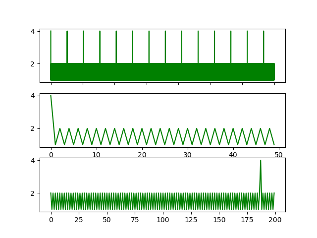
Inspecting the routing channels of the special events, we find that the routing channel numbers are 4, 0, and 2. The 4 marks the beginning of a new frame. The 0 the beginning of a new line and the 2 the end of a line.

fig, ax = plt.subplots(3, 1, sharey=False)
plt.setp(ax[0].get_xticklabels(), visible=False)
ax[0].plot(c[special_events][:7000], 'g')
ax[1].plot(c[special_events][:50], 'g')
ax[2].plot(c[special_events][len(c[special_events])-200:], 'g')
plt.show()

CLSM marker (Leica)

Below, an analysis of the frame and line marker is briefly outlined for a Leica SP8 dataset.

e = tttr_leica.event_types
c = tttr_leica.routing_channels
t = tttr_leica.macro_times
m = tttr_leica.micro_times

The routing channels are inspected to determine the actual channel numbers of the detectors. A bincount over the channel numbers determines how often a channel occurs in the data stream. Look for used channels

y = np.bincount(c)
print(y)
plt.plot(y)
plt.show()

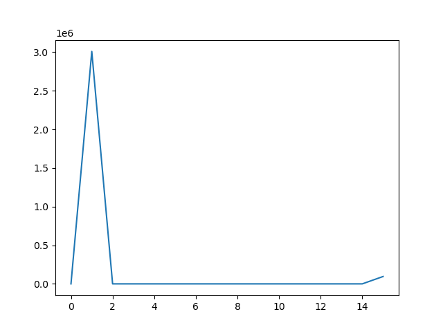
[      0 3009504       0       0       0       0       0       0       0
       0       0       0       0       0       0   95325]

In the dataset two channels were populated (channel 1 and channel 15). For the measurements only a single detector was used. Hence, likely, channel 15 was used to encode other information.

• 1 - 3009504

• 15 - 95325

Note

Usually, the TTTR records utilize the event type to distinguish markers from photons. Leica decided to use the routing channel number to identify markers.

Based on these counts, channel 15 very likely identifies the markers. The number of events 95325 closely matches a multiple of 2 (95325 = 93 * 512 + 3). Note, there are 1024 lines in the images, 4 images in the file.

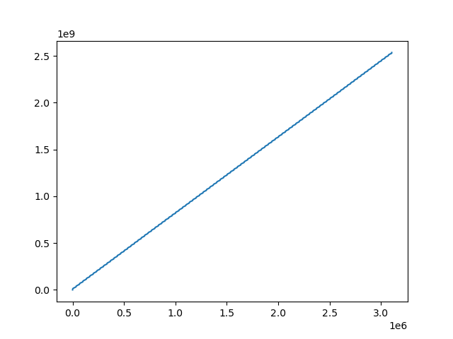
By looking at the macro time one can also finds that there are 93 images in the file, as intensity within the image in non-uniform. Hence, the macro time fluctuates.

plt.plot(tttr_leica.macro_times)
plt.show()

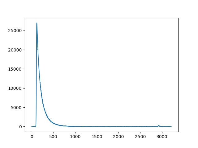
To make sure that the routing channel 1 is indeed a detection channels, one can create (in a time-resolved experiment) a bincount of the associated micro times.

m_ch_1 = m[np.where(c == 1)]
y = np.bincount(m_ch_1)
plt.plot(y)
plt.show()

Next, to identify if in addition to the channel number 15 the markers are identified by non-photon event marker we make a bincount of the channel numbers, where the event type is 1 (photon events have the event type 0, non-photon events have the event type 1).

y = np.bincount(c[np.where(e == 1)])
plt.plot(y)
plt.show()

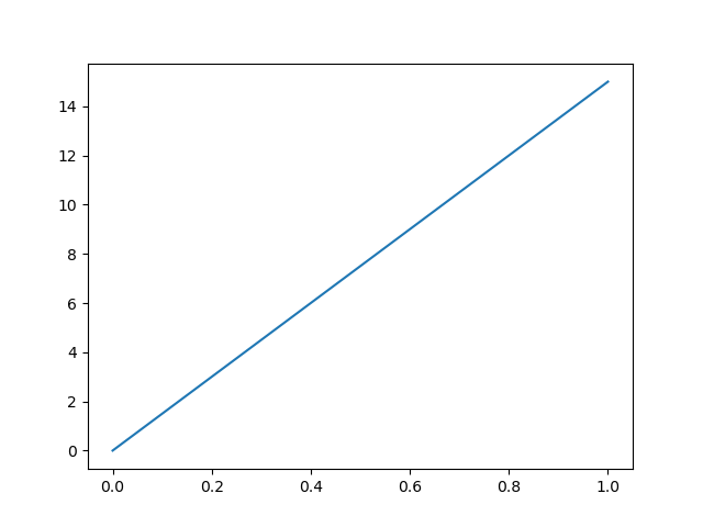
To sum up, channel 1 is a routing channels of the detector. Channel 15 is the routing channel used to inject the special markers. Next, we inspect the micro time and the macro time of the events registered by the routing channel 15.

The plot of the micro times for the events of the routing channel 15 reveals, that the micro time is either 1, 2, or 4. A more close inspection reveals that a micro time value of 1 is always succeeded by a micro time value of 2.

m_ch_15 = m[np.where(c == 15)]
plt.plot(m_ch_15)
plt.show()

A micro time value of 4 is followed by a micro time value of 1. This means, that the micro time encodes the frame marker and the line start/stop markers.

• micro time 1 - line start

• micro time 2 - line stop

• micro time 4 - frame start

Note

The first frame does not have a frame start.

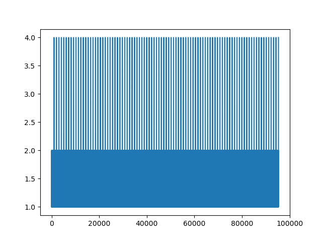
Next, the macro time of the events where the routing channel number equals 15 is inspected. As anticipated, the macro time increases on first glance continuously. On closer inspection, however, steps in the macro time are visible.

plt.plot(t[np.where(c == 15)])
plt.show()

To sum up, in the Leica SP8 PTU files

1. line and frame markers are treated as regular photons.

2. the line and frame markers are identified by the routing channel number 15

3. the type of a marker is encoded in the micro time of channels with a channel number 15

Note

Usually, the TTTR records utilize the event type to distinguish markers from photons. Here, Leica decided to use the routing channel number to identify markers. When opening an image in tttrlib this special case is considered by specifying the reading routine.

Conclusion

It is not always fully documented how a manufacturer of a microscope encodes # laser scanning microscopy data in TTTR files. Often it is unclear how the frame and line marker are integrated into the event data stream. The encoding of the frame and line markers of the custom setup is more widespread. Thus, it is the default when reading CLSM data. Moreover, the meta data (which was not discussed here) contains additional (optional) information on how to read/process the photon stream.