Lifetime analysis

Fit a decay to photons in pixel to determine a mean fluorescence lifetime.

Import necessary libraries

import tttrlib
import numpy as np
import pylab as plt

The fit operates on a parallel and a perpendicular detection channel. Here we define the channel numbers of the two channels and read the tttr data of the clsm experiment. Moreover, we define a binning factor that is used to coarsen the micro time.

ch_p = [0]
ch_s = [1]
binning_factor = 64
minimum_n_photons = 30

fn_clsm = '../../tttr-data/imaging/pq/ht3/crn_clv_img.ht3'
data = tttrlib.TTTR(fn_clsm)

Next we create two CLSM container for the parallel and perpendicular channel and stack frames to have more photons in each pixel.

clsm_p = tttrlib.CLSMImage(data, channels=ch_p, fill=True)
clsm_s = tttrlib.CLSMImage(data, channels=ch_s, fill=True)
clsm_p.stack_frames()
clsm_s.stack_frames()

We determine instrument response function in parallel and perpendicular detection channels.

fn_irf = '../../tttr-data/imaging/pq/ht3/crn_clv_mirror.ht3'
irf_tttr = tttrlib.TTTR(fn_irf)
irf_data_p: tttrlib.TTTR = irf_tttr[irf_tttr.get_selection_by_channel(ch_p)]
irf_data_s: tttrlib.TTTR = irf_tttr[irf_tttr.get_selection_by_channel(ch_s)]

We get micro time histograms for the IRF and stack the histograms

irf_p, t = irf_data_p.get_microtime_histogram(binning_factor)
irf_s, _ = irf_data_s.get_microtime_histogram(binning_factor)
irf = np.hstack([irf_p, irf_s])

Settings for MLE

settings = {
    'dt': data.header.micro_time_resolution * 1e9 * binning_factor,
    'g_factor': 1.0, 'l1': 0.05, 'l2': 0.05,
    'convolution_stop': -1,
    'irf': irf,
    'period': 32.0,
    'background': np.zeros_like(irf)
}

The settings are used to initialize an instance of the class Fit23. A dataset is fitted by calling an instance of Fit23 using the data, an array of the initial values of the fitting parameters, and an array that specifies which parameters are fixed.

fit23 = tttrlib.Fit23(**settings)
tau, gamma, r0, rho = 3.2, 0.05, 0.38, 10.0
x0 = np.array([tau, gamma, r0, rho])
fixed = np.array([0, 0, 1, 0])

We iterate over all pixels in the image and apply the fit to pixels where we have at certain minimum number of photons.

intensity = clsm_p.intensity
micro_times = data.micro_times // binning_factor
n_channels = data.header.number_of_micro_time_channels // binning_factor
tau = np.zeros_like(intensity, dtype=np.float32)
rho = np.zeros_like(intensity, dtype=np.float32)
n_frames, n_lines, n_pixel = clsm_p.shape

# These loops are not very fast but get the job done
import time
time_start = time.time()
for i in range(n_frames):
    for j in range(0, n_lines, 1):
        for k in range(n_pixel):
            idx_p = clsm_p[i][j][k].tttr_indices
            idx_s = clsm_s[i][j][k].tttr_indices
            n_p = len(idx_p)
            n_s = len(idx_s)
            if n_p + n_s < minimum_n_photons:
                continue
            hist = np.hstack(
                [
                    np.bincount(micro_times[idx_p], minlength=n_channels),
                    np.bincount(micro_times[idx_s], minlength=n_channels)
                ]
            )
            r = fit23(hist, x0, fixed)
            tau[i, j, k] = r['x'][0]
time_stop = time.time()
print("Elapsed time:", time_stop - time_start)

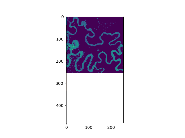
plt.imshow(tau[0], vmin=0, vmax=5)
plt.show()

plt.hist(tau[0].flatten(), 131, range=(0.01, 5))
plt.show()

Elapsed time: 28.92492961883545