Phasor analysis of images

Introduction

Changing the data representation from the classical time delay histogram to the phasor representation provides a global view of the fluorescence decay at each pixel of an image. In the phasor representation we can easily recognize the presence of different molecular species in a pixel or the occurrence of fluorescence resonance energy transfer. The analysis of the fluorescence lifetime imaging microscopy (FLIM) data in the phasor space is done observing clustering of pixels values in specific regions of the phasor plot rather than by fitting the fluorescence decay using exponentials. The analysis is instantaneous since is not based on calculations or nonlinear fitting. The phasor approach has the potential to simplify the way data are analyzed in FLIM, paving the way for the analysis of large data sets and, in general, making the FLIM technique accessible to the nonexpert in spectroscopy and data analysis [DIGMAN2008L14].

from __future__ import print_function
import tttrlib

import pylab as plt
import numpy as np

Read data of the CLSM image

data = tttrlib.TTTR('../../tttr-data/imaging/pq/ht3/crn_clv_img.ht3')
# Macro time in header missing
ht3_reading_parameter = {
    "marker_frame_start": [4],
    "marker_line_start": 1,
    "marker_line_stop": 2,
    "marker_event_type": 1,
    "n_pixel_per_line": 256,
    "reading_routine": 'default',
    "channels": [0, 1],
    "fill": True,
    "tttr_data": data,
    "skip_before_first_frame_marker": True
}
image = tttrlib.CLSMImage(**ht3_reading_parameter)

stack_frames = True
minimum_number_of_photons = 60

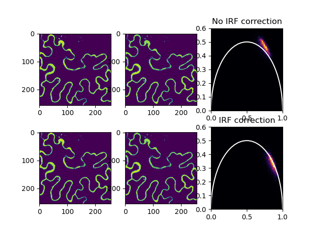
# No IRF correction
phasor = image.get_phasor(
    tttr_data=data,
    stack_frames=stack_frames,
    minimum_number_of_photons=minimum_number_of_photons
)

n_frames = 1 if stack_frames else image.n_frames
phasor_1d = phasor.reshape((n_frames * image.n_lines * image.n_pixel, 2))
phasor_x, phasor_y = phasor[:, :, :, 0], phasor[:, :, :, 1]
phasor_x_1d_1, phasor_y_1d_1 = phasor_1d.T[0], phasor_1d.T[1]

ssas IRF correction

data_mirror = tttrlib.TTTR('../../tttr-data/imaging/pq/ht3/crn_clv_mirror.ht3')
data_irf = data_mirror[data_mirror.get_selection_by_channel([0, 1])]
phasor = image.get_phasor(
    tttr_irf=data_irf,
    tttr_data=data,
    stack_frames=stack_frames,
    minimum_number_of_photons=minimum_number_of_photons
)

n_frames = 1 if stack_frames else image.n_frames
phasor_1d = phasor.reshape((n_frames * image.n_lines * image.n_pixel, 2))
phasor_x, phasor_y = phasor[:, :, :, 0], phasor[:, :, :, 1]
phasor_x_1d_2, phasor_y_1d_2 = phasor_1d.T[0], phasor_1d.T[1]

Plot histogram of pixels phasors

hist_settings = {
    'bins': 101,
    'range': ((0, 1), (0, 0.6)),
    'cmap': 'inferno'
}
circle_settings = {
    "xy": (0.5, 0),
    "radius": 0.5,
    "linewidth": 1.5,
    "fill": False,
    "color": 'w'
}

fig, ax = plt.subplots(nrows=2, ncols=3)
ax[0, 2].set(xlim=(0, 1), ylim=(0, 0.6))
ax[0, 2].hist2d(phasor_x_1d_1, phasor_y_1d_1, **hist_settings)
ax[0, 0].imshow(phasor_x[0, :, :])
ax[0, 1].imshow(phasor_y[0, :, :])
ax[1, 2].set(xlim=(0, 1), ylim=(0, 0.6))
ax[1, 2].hist2d(phasor_x_1d_2, phasor_y_1d_2, **hist_settings)
ax[1, 0].imshow(phasor_x[0, :, :])
ax[1, 1].imshow(phasor_y[0, :, :])

a_circle = plt.Circle(**circle_settings)
ax[1, 2].add_artist(a_circle)
a_circle = plt.Circle(**circle_settings)
ax[0, 2].add_artist(a_circle)

ax[0, 2].set_title('No IRF correction')
ax[1, 2].set_title('IRF correction')

plt.show()

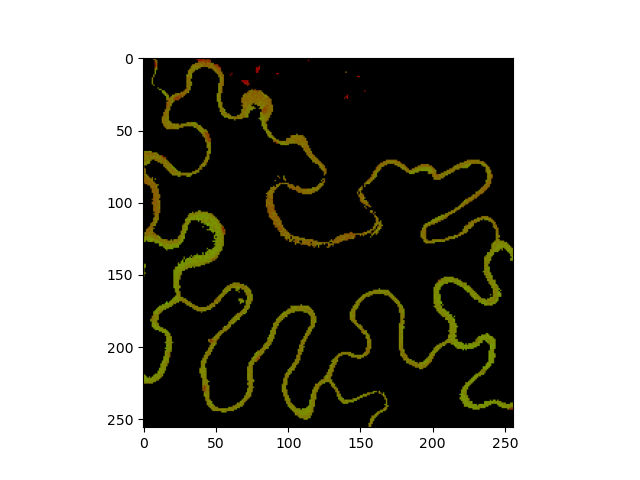
The both phasor values can be inspected by mapping them to colors.

phasor_clr = np.zeros((phasor.shape[1], phasor.shape[2], 3))
phasor_xc = np.clip(phasor_x * 0.59, 0, 1)
phasor_yc = np.clip(phasor_y * 1.45, 0, 1)
phasor_clr[:, :, 0] = phasor_xc
phasor_clr[:, :, 1] = phasor_yc
plt.imshow(phasor_clr, vmin=0.6, vmax=0.8)
plt.show()