Image-based segmentation of FLIM data

Overview

In live-cell imaging, the conformation or the oligomeric state of biomolecules can depend on their cellular location. In this application example we combine image segmentation with fluorescence-lifetime based analysis and generate fluorescence intensity decays of molecular sub-ensembles to resolve molecular states of the studied protein of interest for different cellular compartments. We segment multi-parameter fluorescence image spectroscopy (MFIS) data into nucleus, cytoplasm and vesicles-like structures.

1. Data Loading

2. Create CLSM image container

3. Pulsed interleaved excitation

4. Intensity imaging

5. Micro time imaging

6. Define pixel classes by image segmentation

7. Apply pixel classes for analysis

import tttrlib
import numpy as np
import matplotlib.pyplot as plt
import skimage as ski
import skimage.filters
import skimage.morphology
import skimage.util
import scipy
import scipy.ndimage


def plot_images(images, titles, cmaps=None, **kwargs):
    # Define convenience function for plotting
    if cmaps is None:
        cmaps = ['viridis'] * len(images)
    if titles is None:
        titles = [''] * len(images)
    fig, ax = plt.subplots(**kwargs)
    if not isinstance(ax, list):
        ax = np.array([ax])
    ax = ax.flatten()
    for i, img in enumerate(images):
        im = ax[i].imshow(img, cmap=cmaps[i])
        ax[i].set_title(titles[i])
        fig.colorbar(im, ax=ax[i], fraction=0.046, pad=0.04)
    return fig, ax

1. Loading data and creating the intensity images

First, read the TTTR data. Define used channels

filename_data = '../../tttr-data/imaging/pq/ht3/mGBP_DA.ht3'
tttr_data = tttrlib.TTTR(filename_data)

print("Used routing channels:", tttr_data.used_routing_channels)
green_ch = [0, 1]
red_ch = [4, 5]
sum_all = green_ch + red_ch

Used routing channels: [4 5 0 1 2]

3. Pulsed interleaved excitation

Split the data into prompt and delay. For a more detailed description see plot_pie_flim.py

filename_irf = '../../tttr-data/imaging/pq/ht3/mGBP_IRF.ht3'
irf = tttrlib.TTTR(filename_irf)
tttr_irf_green = irf.get_tttr_by_channel(green_ch)
tttr_irf_red = irf.get_tttr_by_channel(red_ch)
tttr_green = tttr_data.get_tttr_by_channel(green_ch)
tttr_red = tttr_data.get_tttr_by_channel(red_ch)
prompt_range = 0, 11000
delay_range = 11000, 25000

2. Create CLSM image container

# In the green channel we use all photons
clsm_green = tttrlib.CLSMImage(tttr_data=tttr_data, channels=green_ch)
clsm_red_prompt = tttrlib.CLSMImage(tttr_data=tttr_data, channels=red_ch, micro_time_ranges=[prompt_range])
clsm_red_delay = tttrlib.CLSMImage(tttr_data=tttr_data, channels=red_ch, micro_time_ranges=[delay_range])

3. Intensity imaging

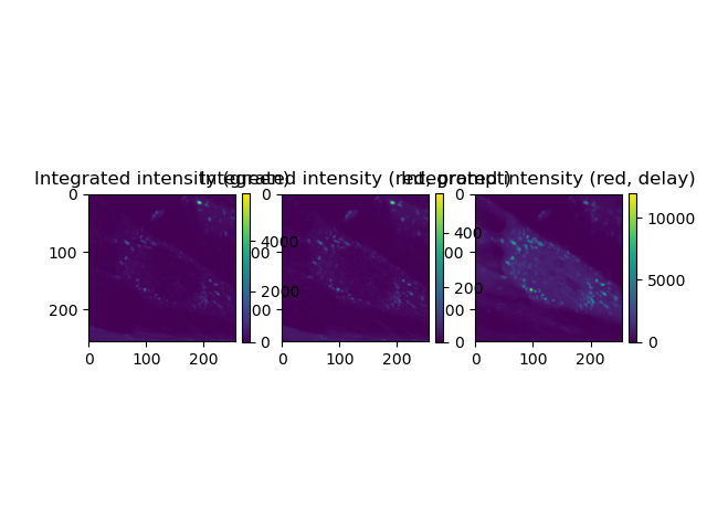
Fills the CLSM image container with intensities An intensity image the number of counts in a pixel corresponds to the number of photons Red intensity is toatal intenstiy, ie, prompt + delayed excitation Fig. 4B Green, red prompt, red delay Sum over all frames The intensity images are a time-series (multiple frames). We sum over all frames to improve the counting statistics Note: image shape is in the order of t-y-x, thus summation of over axis=0 results in generating the t-projection

SUM_green = clsm_green.intensity.sum(axis=0)
SUM_red_prompt = clsm_red_prompt.intensity.sum(axis=0)
SUM_red_delay = clsm_red_delay.intensity.sum(axis=0)

fig, _ = plot_images(
    [SUM_green, SUM_red_prompt, SUM_red_delay],
    ncols=3, nrows=1,
    titles=[
        'Integrated intensity (green)',
        'Integrated intensity (red, prompt)',
        'Integrated intensity (red, delay)',
    ]
)
fig.show()

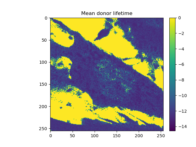
Lifetime analysis

mean_tau_green = clsm_green.get_mean_lifetime(
    tttr_data,
    minimum_number_of_photons=20,
    stack_frames=True,
    tttr_irf=tttr_irf_green
)
fig, _ = plot_images(
    [mean_tau_green[0]],
    ncols=1, nrows=1,
    titles=[
        'Mean donor lifetime'
    ]
)
fig.show()

7. Image segmentation

# Next, we use the generated intensity image and use standard image segmentation
# techniques like Median or Gaussian filtering, Li- or Otsu-based thresholding to
# separate the three regions of interest: cytoplasm, vesicles and nucleus.
# At the end these segmentations represent binary masks, which are filled with "1/TRUE" in
# the region of interest and "0/FALSE" outside.

7.1 Segmentation of the vesicles

We start with the segmentation of the vesicles. Here, first a Gaussian smoothing with a size of 1 sigma is applied, followed by thresholding using the method of Otsu. Finally, objects with a size smaller than 5 pixels are removed.

sigma_vesicles = 1  # radius for Gaussian smoothing
min_vesicle_size = 5  # give minimal vesicle size in pixel
# Calculate intensity sum over all detection channels
# This facilitates the segmentation due to higher SNR
int_all_channel = clsm_green.intensity + clsm_red_prompt.intensity + clsm_red_delay.intensity
filled_frames = 0, 378

binary_img_vesicles = []
for image in range(*filled_frames):
    input_img = int_all_channel[image,:,:]
    # A. Gaussian filtering
    gaussian_img = ski.filters.gaussian(input_img, sigma=sigma_vesicles)
    thresh_vesicles = ski.filters.threshold_otsu(gaussian_img)  # B. Determine Otsu threshold for each frame
    binary_temp = gaussian_img >= thresh_vesicles  # C. Intensities larger than threshold = TRUE /1
    # D. Remove small objects
    cleaned_image = ski.morphology.remove_small_objects(binary_temp, min_vesicle_size)
    binary_img_vesicles.append(cleaned_image)

vesicle_mask = (np.array(binary_img_vesicles, dtype=np.ubyte))

7.2 Segmentation of the cytoplasm

Next, the cytoplasm is segmented. Here, first a median filtering with a disk size of 3 pixel is applied. This is followed by thresholding using the method of Otsu. However, for later frames direct usage of the Otsu threshold selected too much of background, thus we slightly increase the threshold by multiplying with 1.03 (Otsu_scaling_factor) In the final steps, first small holes inside the cytoplasm area are closed, followed by the removal of small detected areas outside the main cell. Here, a minimal size threshold of 10’000 pixel is applied.

disk_size_cyto = 3  # smoothing radius in pixel for median filtering
otsu_scaling_factor = 1.03  # increase Otsu threshold by multiplication with this factor
minimal_size = 10000  # give minimal cytoplasm size in pixel

binary_img_cytoplasm = []
for image in range(*filled_frames):
    input_img = int_all_channel[image,:,:]
    # A. Median filtering
    median_img = ski.filters.median(input_img, ski.morphology.disk(disk_size_cyto))
    thresh_cyto = ski.filters.threshold_otsu(median_img)  # B. Determine Otsu threshold for each frame
    binary_temp = median_img >= thresh_cyto*otsu_scaling_factor  # C. Intensities larger than threshold = TRUE /1
    # D. Fill holes in the cytoplasm
    bool_img = scipy.ndimage.binary_fill_holes(binary_temp)
    segmentation_filled = np.copy(bool_img.astype(np.uint8))
    # E. Remove small speckles outside the large cell
    small_aggregates_removed = ski.morphology.area_closing(ski.util.invert(segmentation_filled), area_threshold=minimal_size)
    final_segmentation = ski.util.invert(small_aggregates_removed)
    binary_img_cytoplasm.append(final_segmentation)
cytoplasm_mask = (np.array(binary_img_cytoplasm, dtype=np.ubyte))

7.3 Segmentation of nucleus

Finally, the nucleus is segmented. In contrast to the cytoplasm and vesicles, here only the green intensity image is used as input as here the contrast between cytoplasm/vesicles region and nucleus seemed largest. Please note that the nucleus can be best seen as “region in cytoplasm but without vesicles”. The segmentation of the nucleus thus proves to be a challenge. We first apply a Gaussian smoothing with a radius of 2 sigma, followed by thresholding using the method of Li. The thresholded image is dilated, holes inside the nucleus filled and small areas outside removed. Next all left-overs outside the cytoplasmic (i.e. body of the cell) are removed by multiplying with the generated cytoplasm mask, followed by another round of dilation to make the nucleus “smoother”. Finally, as the nucleus is characterized by being outside the way of the diffusing vesicles, we average the such obtained nucleus and generate an average nucleus by summing over all 400 frames and threshold this projection using the method of Otsu.

sigma_nucleus = 2  # radius for Gaussian filtering
dilation_radius = 2  # for dilation operation
minimal_hole_size = 1000  # minimal area size (smaller areas will be removed)
minimal_nucleus_size = 2000 # minimal nucleus size

binary_img_nucleus = []
int_green = clsm_green.intensity
for image in range(*filled_frames):
    input_img = int_green[image,:,:]
    input_img_cytoplasm = cytoplasm_mask[image,:,:]
    # A. Gaussian img
    gaussian_img_nucleus = ski.filters.gaussian(input_img, sigma=sigma_nucleus)
    # B. Li-thresholding
    li_threshold = ski.filters.threshold_li(gaussian_img_nucleus)
    thresholded_image = gaussian_img_nucleus > li_threshold
    # C. Dilation
    dilated_segmentation = ski.morphology.dilation(thresholded_image, ski.morphology.disk(dilation_radius))
    # D. Fill holes
    bool_img = scipy.ndimage.binary_fill_holes(dilated_segmentation)
    segmentation_filled = np.copy(bool_img.astype(np.uint8))
    # E Remove small areas
    small_areas_removed = ski.morphology.area_closing(ski.util.invert(segmentation_filled), area_threshold=minimal_nucleus_size)
    # F. Combine with cytoplasm by multiplication of binary images
    combination = np.zeros(small_areas_removed.shape, dtype=np.uint)
    combination = input_img_cytoplasm * (small_areas_removed - 254)
    # G. Remove small areas at the cytoplasm border
    cleaned_combination = ski.morphology.area_closing(ski.util.invert(combination), area_threshold=minimal_nucleus_size)
    # H. dilate Nucleus to make more "smooth"
    dilated_combination = ski.morphology.dilation(ski.util.invert(cleaned_combination), ski.morphology.disk(dilation_radius))
    binary_img_nucleus.append(dilated_combination)

# I. Average over all frames to get a smoother nucleus
averaged_img_nucleus = np.sum(binary_img_nucleus, axis=0).astype(dtype=np.int64)
Otsu_thresh = ski.filters.threshold_otsu(averaged_img_nucleus)
thresholded_img = averaged_img_nucleus > Otsu_thresh
# J. Maybe required to removed smaller stuff
nucleus_mask_avg = ski.morphology.remove_small_objects(thresholded_img, min_size=minimal_nucleus_size)

In the next two steps, we clean up the cytoplasm and vesicles masks. First, we remove the nucleus and vesicles from the cytoplasm, and second we remove the vesicles inside the nucleus region - if any- and the vesicles beloging to the neighboring cell from the vesicles mask.

7.4 Remove nucleus and vesicles from cytoplasm

We invert the average nucleus mask and multiply with each frame, followed by inverting the vesicles mask and frame-wise multiplication. Remember that all masks are filled with 0 and 1, thus 0*0 or 0*1 = 0, only those regions, where both, in the cytoplasm mask and the inverted mask, the value 1 is given, stay 1.

inv_nucleus = ski.util.invert(nucleus_mask_avg)  # Invert nucleus_mask

cytoplasm_wo_nucleus_list = []  # Apply nucleus mask on cytoplasm
for image in range(cytoplasm_mask.shape[0]):
    input_img = cytoplasm_mask[image,:,:]
    temp_cyto = input_img * inv_nucleus
    cytoplasm_wo_nucleus_list.append(temp_cyto)

cytoplasm_wo_nucleus = (np.array(cytoplasm_wo_nucleus_list, dtype=np.ubyte))

inv_vesicles = ski.util.invert(vesicle_mask) - 254  # Invert vesicle_mask

cytoplasm_wo_nucleus_vesicles = []  # Apply vesicle mask on cytoplasm_wo_nucleus
for image in range(cytoplasm_mask.shape[0]):
    input_img = cytoplasm_wo_nucleus[image,:,:]
    input_img_inv_vesicle = inv_vesicles[image,:,:]
    temp_cyto2 = input_img * input_img_inv_vesicle
    cytoplasm_wo_nucleus_vesicles.append(temp_cyto2)

# Final cytoplasm mask:
mask_cytoplasm = (np.array(cytoplasm_wo_nucleus_vesicles, dtype=np.ubyte))

7.5 Remove vesicles in nucleus regions and outside cell of interest

Here, the same strategy as for the cleaned up cytoplasm is used. First vesicles inside the nucleus are removed, followed by those outside the main cell by multiplying with inverted masks.

vesicles_wo_nucleus_list = []  # Apply nucleus mask
for image in range(vesicle_mask.shape[0]):
    input_img = vesicle_mask[image,:,:]
    temp_vesicle = input_img * inv_nucleus
    vesicles_wo_nucleus_list.append(temp_vesicle)

vesicles_wo_nucleus = (np.array(vesicles_wo_nucleus_list, dtype=np.ubyte))

vesicles_in_cytoplasm = []  # Apply cytoplasm mask on nucleus-free vesicles
for image in range(vesicle_mask.shape[0]):
    input_img_vesicle = vesicles_wo_nucleus[image,:,:]
    input_img_cytoplasm = cytoplasm_wo_nucleus[image,:,:]
    temp_vesicle_in_cyto = input_img_vesicle * input_img_cytoplasm
    vesicles_in_cytoplasm.append(temp_vesicle_in_cyto)

# Final vesicles mask:
mask_vesicles = (np.array(vesicles_in_cytoplasm, dtype=np.ubyte))

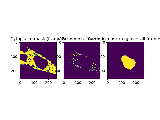
fig, ax = plt.subplots(1, 3, sharex=False, sharey=False)
im = ax[0].imshow(mask_cytoplasm[0])
ax[0].set_title('Cytoplasm mask (frame 0)')
im = ax[1].imshow(mask_vesicles[0])
ax[1].set_title('Vesicle mask (frame 0)')
im = ax[2].imshow(nucleus_mask_avg)
ax[2].set_title('Nucleus mask (avg over all frames)')
plt.show()

8. Apply pixel classes for analysis

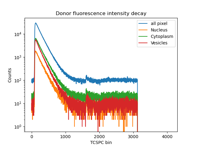
Apply generated masks to reconstruct green intensity decays Now we used the generated masks for our three regions of interest and group the pixels belonging to each class. This procedure is applied to every individual frame. Then, based on the micro time information in each pixel the photon arrival time histogram can be reconstructed. However, first we ignore our masks and generate the mean arrival time image summed over all frames. Next, the summed decays for all pixel and the three pixel classes are generated.

# generate decays for unmasked pixel
n_frames, n_lines, n_pixel = clsm_green.shape
pseudo_mask = np.ones((n_frames, n_lines, n_pixel), dtype=np.uint8)
kw = {
    "tttr_data": tttr_data,
    "mask": pseudo_mask,  # Here a mask filled with all 1 is used
    "tac_coarsening": 8,  # binning of the micro times
    "stack_frames": True  # TRUE = all frames are summed up
}
decay_all = clsm_green.get_decay_of_pixels(**kw)
sum_decay_all = decay_all.sum(axis=0)

# Generate decay from masked pixels for cytoplasm, nucleus and vesicles
# Caution: for nucleus only single average image mask was generated
# "multiply" 400x to have a mask for each frame
final_cytoplasm = np.zeros((n_frames, n_lines, n_pixel), dtype=np.uint8)
for i in range(*filled_frames):
    final_cytoplasm[i] = mask_cytoplasm[i]
kw_cytoplasm = {
    "tttr_data": tttr_data,
    "mask": final_cytoplasm,  # cyotplasm mask
    "tac_coarsening": 8,
    "stack_frames": True
}
decay_cytoplasm = clsm_green.get_decay_of_pixels(**kw_cytoplasm)
sum_decay_cytoplasm = decay_cytoplasm.sum(axis=0)

final_vesicles = np.zeros((n_frames, n_lines, n_pixel), dtype=np.uint8)
for i in range(*filled_frames):
    final_vesicles[i] = mask_vesicles[i]
kw_vesicles = {
    "tttr_data": tttr_data,
    "mask": final_vesicles,  # vesicles mask
    "tac_coarsening": 8,
    "stack_frames": True
}
decay_vesicles = clsm_green.get_decay_of_pixels(**kw_vesicles)
sum_decay_vesicles = decay_vesicles.sum(axis=0)

# Caution: for nucleus only single average image mask was generated
# "multiply" 400x to have a mask for each frame
nucleus_mask = np.zeros((n_frames, n_lines, n_pixel), dtype=np.uint8)
for i in range(n_frames):
    nucleus_mask[i] = nucleus_mask_avg
kw_nucleus = {
    "tttr_data": tttr_data,
    "mask": nucleus_mask,  # nucleus mask
    "tac_coarsening": 8,
    "stack_frames": True
}
decay_nucleus = clsm_green.get_decay_of_pixels(**kw_nucleus)
sum_decay_nucleus = decay_nucleus.sum(axis=0)

fig, ax = plt.subplots(1, 1, sharex=False, sharey=False)
ax.semilogy(sum_decay_all, label='all pixel')
ax.semilogy(sum_decay_nucleus, label='Nucleus')
ax.semilogy(sum_decay_cytoplasm, label='Cytoplasm')
ax.semilogy(sum_decay_vesicles, label='Vesicles')
ax.legend()
ax.set(xlabel='TCSPC bin', ylabel='Counts',
             title='Donor fluorescence intensity decay')
plt.show()