Tutorial: Image construction

Below, using a few lines of python code it is outlined how CLSM images can be constructed. For productive uses tttrlib provides a set of functions to create images based on CLSM TTTR data implemented in C/C++. To describe how this is actually implemented, it is outlined below in Python only using basic the basic functionality of tttrlib. The presented outline presented below may serve to understand how the image construction in CLSM work and is not intended for productive use.

For any productive applications it is recommended to use the built-in tttrlib CLSM functions.

import tttrlib
import numpy as np
import pylab as p
import numba as nb


@nb.jit(nopython=True)
def count_marker(channels, event_types, marker, event_type):
    n = 0
    for i, ci in enumerate(channels):
        if (ci == marker) and (event_types[i] == event_type):
            n += 1
    return n


@nb.jit(nopython=True)
def find_marker(channels, event_types, maker, event_type=1):
    r = list()
    for i, ci in enumerate(channels):
        if (ci == maker) and (event_types[i] == event_type):
            r.append(i)
    return np.array(r)

In the example above, first the number of frames are counted. Next, the number of start line events are counted. In the example, there are overall 41 frames are present in the file each having 256 lines. As the last frame is often incomplete (see Figure above) the last frame is neglected (41 - 1 = 40). With the script above, the number of frames n_frames and the number of lines per frame n_lines_per_frame is determined. Next, the number of pixel per line n_pixel can be freely defined. Based on the time the laser spends in each line, the duration per pixel (the laser is constantly scanning) needs to be calculated. Here, there are two options: 1) either the total time from the beginning of each new line (line start) to the beginning of the next line is considered as a line or 2) the time between the line start and the line stop is considered as the time base to calculate the pixel duration. In the first case, the back movement of the laser to the line start can be visualized in the image. In the later case, only the valid region where the laser scans over the sample is visualized. For most applications the later approach is useful. To understand the microscope laser scanner the former approach is more useful. Above, line_duration_valid is the time the laser spends in every of the lines in a valid region and line_duration_total is the total time the laser spends in a line including the rewind to the line beginning. Above, n_pixel is the freely defined number of pixels per line and pixel_duration is the duration of every pixel. With the number of frames n_frames, the number of pixels n_pixel, and the number of lines n_lines_per_frame it is clear how much the memory for an image needs to be can be allocated and with the defined number of pixels per line the duration for the pixel can be calculated for all the lines of the frames.

With these numbers an image for a certain set of detector channels detector_channels can be calculated. Below this is by the function make_image.

@nb.jit(nopython=True)
def make_image(
        c, m, t, e,
        n_frames, n_lines, pixel_duration,
        channels,
        frame_marker=4,
        line_start=1,
        line_stop=2,
        n_pixel=None,
        tac_coarsening=32,
        n_tac_max=2**15):
    if n_pixel is None:
        n_pixel = n_lines  # assume squared image

    n_tac = int(n_tac_max // tac_coarsening)
    image = np.zeros(
        (int(n_frames), int(n_lines), int(n_pixel), int(n_tac)),
        dtype=np.uint16
    )
    # iterate through all photons in a line and add to image

    frame = -1
    current_line = 0
    time_start_line = 0
    invalid_range = True
    mask_invalid = True
    for i in range(len(c)):
        ci, mi, ti, ei = c[i], m[i], t[i], e[i]
        if ei == 1:  # marker
            if ci == frame_marker:
                frame += 1
                current_line = 0
                if frame < n_frames:
                    continue
                else:
                    break
            elif ci == line_start:
                time_start_line = ti
                invalid_range = False
                continue
            elif ci == line_stop:
                invalid_range = True
                current_line += 1
                continue
        elif ei == 0:  # photon
            in_channels = False
            for v in channels:
                if v == ci:
                    in_channels = True
            if in_channels and (not invalid_range or not mask_invalid):
                pixel = int((ti - time_start_line) // pixel_duration[current_line])
                if pixel < n_pixel:
                    tac = mi // tac_coarsening
                    image[frame, current_line, pixel, tac] += 1
    return image


events = tttrlib.TTTR('../../tttr-data/imaging/pq/ht3/pq_ht3_clsm.ht3', 1)
e = events.get_event_type()
c = events.get_routing_channel()
t = events.get_macro_times()
m = events.get_micro_times()

Before creating an image the channel numbers of the frame and the line markers need to be determined. For the example that is shown above the frame, line start, and line stop markers are 4, 1, and 2, respectively. Next, the TTTR data needs to be loaded into memory, the number of frames, and the number of lines need to be determined in order to allocate memory for the image. In CLSM the number of pixels per line can be arbitrarily defined, as the laser beam is continuously displaced and the fluorescence of the sample is continuously recorded. Hence, the main experimental determinants of the image size in memory are the number of frames and the number of line scans per frame. Usually, the number of line scans per frame is constant within a TTTR file.

The number of frames can be determined by counting extracting and counting the number of frame markers as shown below.

Note

The channel number of the frame makers (here 4) depends on the experimental setup. Moreover, some setup configurations use “photons” event types to record special events. Different microscopes may use different markers. For common microscopes such as the Leica SP5 and Leica SP8 ready-to-use image processing routines are provided.

frame_marker_list = find_marker(c, e, 4)
line_start_marker_list = find_marker(c, e, 1)
line_stop_marker_list = find_marker(c, e, 2)
n_frames = len(frame_marker_list) - 1 # 41
n_line_start_marker = len(line_start_marker_list) # 10246
n_lines = n_line_start_marker // n_frames # 256
line_duration_valid = t[line_stop_marker_list] - t[line_start_marker_list]
line_duration_total = t[line_start_marker_list[1:]] - t[line_start_marker_list[0:-1]]
n_pixel = 256
pixel_duration = line_duration_valid // n_pixel
line_duration_valid = t[line_stop_marker_list] - t[line_start_marker_list]

image = make_image(
    c, m, t, e,
    n_frames,
    n_lines,
    pixel_duration,
    channels=np.array([0, 1]),
    tac_coarsening=256
)

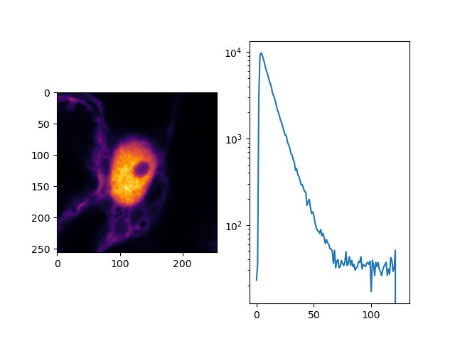
In the example function make_image the an 3D array is created that contains in every pixel a histogram of the micro times. An histogram of the micro time can be displayed by the code shown below:

fig, ax = p.subplots(1, 2)
ax[0].imshow(image.sum(axis=(0, 3)), cmap='inferno')
ax[1].semilogy(image.sum(axis=(0, 1))[128])
p.show()