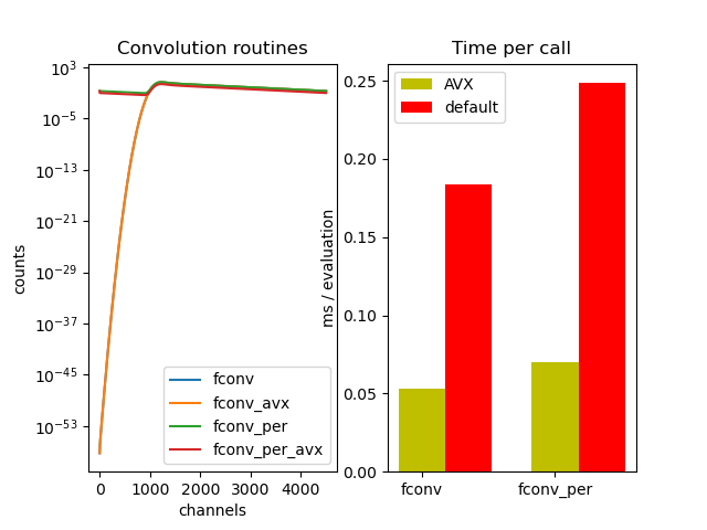
Convolution routines

Overview

In tttrlib there are a set of different convolution routines that can be used to compute fluorescence decays. Most fluorescence decays are linear combinations of exponential decays. Convolutions of such fluorescence decays with instrument response functions can be computed using the routines (fconv, fconv_per, fconv_per_cs, etc.). Here, fconv stands for fast convolution.

For faster convolutions tttrlib provides routines that make use of SIMD (Single Instruction Multiple Data). The SIMD routines use of the AVX2 extension (Advanced Vector Extension). For instance, the routines fconv and fconv_per (periodic convolution) have corresponding SIMD routines named fconv_avx``and ``fconv_per_avx. The SIMD routines compute in parallel the decay in cases the decay is compose of more than a single fluorescence lifetime.

The SIMD AVX make use of AVX2 and FMA (Fused Multiply Add). AVX2 and FMA require CPUs with ‘modern’ instruction sets. Most x86 CPUs that were manufacture since 2012 are supported.

from __future__ import annotations
import tttrlib
import scipy.stats
import time
import numpy as np
import pylab as p

Illustrate the different convolution methods for a computed instrument response function (IRF). Excitation period, i.e., the time between two subsequent excitation pulses Number of micro time channels (usually, linear spacing of micro time channels)

period = 16
n_channels = 4505
irf_position = 4.0
irf_width = 0.25
time_axis = np.linspace(0, period, n_channels)
irf = scipy.stats.norm.pdf(time_axis, loc=irf_position, scale=irf_width)

dt = time_axis[1]-time_axis[0]
lifetime_spectrum = np.array([1., 4, 1., 0.4] * 4)
model = np.zeros_like(irf)
stop = len(irf)
start = 0

Convolution method	function name
Fast convolution	fconv
Fast periodic convolution	fconv_per
Fast convolution (AVX)	fconv_avx
Fast periodic convolution (AVX)	fconv_per_avx
Fast periodic convolution (with stop)	fconv_per_cs
Fast convolution with reference compound	fconv_ref
Convolution of decay curve and IRF	sconv

n_runs = 50
times = list()
times_avx = list()
names = ["fconv", "fconv_per"]
t_start = time.perf_counter()
for _ in range(n_runs):
    tttrlib.fconv(fit=model, irf=irf, x=lifetime_spectrum, start=start, stop=stop, dt=dt)
ex = time.perf_counter() - t_start
times.append(ex)

t_start = time.perf_counter()
for _ in range(n_runs):
    tttrlib.fconv_avx(fit=model, irf=irf, x=lifetime_spectrum, start=start, stop=stop, dt=dt)
ex = time.perf_counter() - t_start
times_avx.append(ex)

t_start = time.perf_counter()  # in seconds
for _ in range(n_runs):
    tttrlib.fconv_per(fit=model, irf=irf, x=lifetime_spectrum, period=period, start=start, stop=stop, dt=dt)
ex = time.perf_counter() - t_start
times.append(ex)

t_start = time.perf_counter()
for _ in range(n_runs):
    tttrlib.fconv_per_avx(fit=model, irf=irf, x=lifetime_spectrum, period=period, start=start, stop=stop, dt=dt)
ex = time.perf_counter() - t_start
times_avx.append(ex)

times = np.array(times) * 1000.0 / n_runs
times_avx = np.array(times_avx) * 1000.0 / n_runs


# make plots
##################
fig, ax = p.subplots(nrows=1, ncols=2, sharex=False)

ax[0].set_title('Convolution routines')
ax[0].set_ylabel('counts')
ax[0].set_xlabel('channels')

model = np.zeros_like(irf)
tttrlib.fconv(fit=model, irf=irf, x=lifetime_spectrum, start=start, stop=stop, dt=dt)
ax[0].semilogy(model, label="fconv")

model_avx = np.zeros_like(irf)
tttrlib.fconv_avx(fit=model_avx, irf=irf, x=lifetime_spectrum, start=start, stop=stop, dt=dt)
ax[0].semilogy(model, label="fconv_avx")

model = np.zeros_like(irf)
tttrlib.fconv_per(fit=model, irf=irf, x=lifetime_spectrum, period=period, start=start, stop=stop, dt=dt)
ax[0].semilogy(model, label="fconv_per")

model = np.zeros_like(irf)
tttrlib.fconv_per_avx(fit=model, irf=irf, x=lifetime_spectrum, period=period, start=start, stop=stop, dt=dt)
ax[0].semilogy(model, label="fconv_per_avx")
ax[0].legend()

# Benchmark
ax[1].set_title('Benchmark')
ax[1].set_ylabel('ms / evaluation')

ind = np.arange(len(times))  # the x locations for the groups
ax[1].set_title('Time per call')
ax[1].set_xticks(ind)
ax[1].set_xticklabels(names)

width = 0.35
ax[1].bar(ind, times_avx, width, color='y', label='AVX')
ax[1].bar(ind + width, times, width, color='r', label='default')
ax[1].legend()

p.show()