MLE fit23: Benchmark

This is a benchmark of fit2x.DecayFit.fit23 that implements an maximum likelihood estimator to determine a fluorescence lifetime and a rotational correlation time for time and polarization resolved fluorescence decays with low photon counts.

In this benchmark fluorescence decays are simulated for a fluorescence lifetime in the range (tau_min, tau_max) with varying number of photons. The simulated and the recovered fluorescence lifetimes are compared.

import tttrlib
import numpy as np
import pylab as plt

np.random.seed(0)

# setup some parameters
tau_min = 0.1
tau_max = 5.0

n_photons_min = 20
n_photons_max = 120
n_photon_step = 2

n_samples = 200

n_channels = 32
irf_position_p = 2.0
irf_position_s = 18.0
irf_width = 0.25
period, g_factor, l1, l2, conv_stop = 32, 1.0, 0.1, 0.1, 31
dt = 0.5079365079365079
np.random.seed(0)

irf_np = np.array([0, 0, 0, 260, 1582, 155, 0, 0, 0, 0,
                   0, 0, 0, 0, 0, 0, 0, 0, 0, 0,
                   0, 0, 0, 0, 0, 0, 0, 0, 0, 0,
                   0, 0, 0, 0, 22, 1074, 830, 10, 0, 0,
                   0, 0, 0, 0, 0, 0, 0, 0, 0, 0,
                   0, 0, 0, 0, 0, 0, 0, 0, 0, 0,
                   0, 0, 0, 0], dtype=np.float64)

bg = np.zeros_like(irf_np)

fit23 = tttrlib.Fit23(
    dt=dt,
    irf=irf_np,
    background=bg,
    period=period,
    g_factor=g_factor,
    l1=l1, l2=l2
)

tau, gamma, r0, rho = 2.0, 0.01, 0.38, 1.22
x0 = np.array([tau, gamma, r0, rho])
fixed = np.array([0, 1, 1, 0])

"""
In this loop the fluorescence decays are simulated and the simulated decays are
fitted.
"""

n_photon_dict = dict()
for n_photons in range(n_photons_min, n_photons_max, n_photon_step):
    tau_sim = list()
    tau_recov = list()
    n_photons = int(n_photons)
    for i in range(n_samples):
        tau = np.random.uniform(tau_min, tau_max)
        # n_photons = int(5./tau * n_photon_max)
        param = np.array([tau, gamma, r0, rho])
        corrections = np.array([period, g_factor, l1, l2, conv_stop])
        model = np.zeros_like(irf_np)
        bg = np.zeros_like(irf_np)
        tttrlib.DecayFit23.modelf(param, irf_np, bg, dt, corrections, model)
        model *= n_photons / np.sum(model)
        data = np.random.poisson(model)
        # This performs a with on the data
        r = fit23(data=data, initial_values=x0, fixed=fixed)
        # print("tau_sim: %.2f, tau_recov: %s" % (tau, r['x'][0]))
        tau_sim.append(tau)
        tau_recov.append(r['x'][0])
        n_photon_dict[n_photons] = {
                'tau_simulated': np.array(tau_sim),
                'tau_recovered': np.array(tau_recov)
        }

devs = list()
for k in n_photon_dict:
    tau_sim = n_photon_dict[k]['tau_simulated']
    tau_recov = n_photon_dict[k]['tau_recovered']
    dev = (tau_recov - tau_sim) / tau_sim
    devs.append(dev)



"""
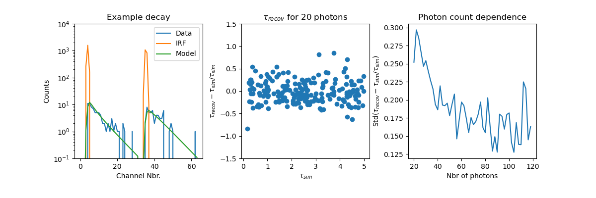
The figures below demonstrate how well the fluorescence lifetime can be recovered.
The left figure displays a typical simulated fluorescence decay. The middle figure
illustrated the relative deviation of the recovered fluorescence lifetime :math:`\tau_{recov}`
from the simulated fluorescence lifetime :math:`\tau_{sim}`. The figure to the right
displays the standard deviation of the relative deviations in dependence of the
number of simulated photons.
"""

fig, ax = plt.subplots(nrows=1, ncols=3, squeeze=True)
fig.set_size_inches(12, 4)
fig.subplots_adjust(bottom=0.2, left=0.125, right=0.9, wspace=0.3)
ax[0].semilogy([x for x in fit23.data], label='Data')
ax[0].semilogy([x for x in fit23.irf], label='IRF')
ax[0].semilogy([x for x in fit23.model], label='Model')
ax[0].set_ylim((0.1, 10000))
ax[0].title.set_text(r'Example decay')
ax[0].set_ylabel(r'Counts')
ax[0].set_xlabel(r'Channel Nbr.')
ax[0].legend()

k = list(n_photon_dict.keys())[0]
tau_sim = n_photon_dict[k]['tau_simulated']
tau_recov = n_photon_dict[k]['tau_recovered']
dev = (tau_recov - tau_sim) / tau_sim
ax[1].title.set_text(r'$\tau_{recov}$ for 20 photons')
ax[1].plot(tau_sim, dev, 'o', label='#Photons: %s' % k)
ax[1].set_ylim((-1.5, 1.5))
ax[1].set_ylabel(r'$\tau_{recov} - \tau_{sim} / \tau_{sim}$')
ax[1].set_xlabel(r'$\tau_{sim}$')

sq_dev = np.array(devs)**2
ax[2].plot(list(n_photon_dict.keys()), np.sqrt(sq_dev.mean(axis=1)))
ax[2].title.set_text(r'Photon count dependence')
ax[2].set_ylabel(r'Std($\tau_{recov} - \tau_{sim} / \tau_{sim}$)')
ax[2].set_xlabel(r'Nbr of photons')
plt.show()