Make a 1D Histogram

tttrlib offers some functions and classes for the creation of histograms. They are part of tttrlib to offer more performance in direct comparison to general purpose routines for analysis methods as Photon Distribution Analysis (PDA) that make heady use of repeated histogram calculations.

Note

These function and classes are not intended as a substitution for more general functions, e.g., offered by NumPy and are less tested. They offer performance advantages for histograms calculated on a logarithmic (log10) scale and a linear scale in direct comparison to NumPy.

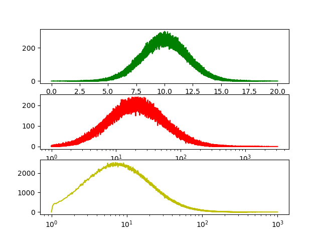
One dimensional histograms

tttrlib supports one dimensional histograms with linear, logarithmic, or arbitrary spaced bins.

#.. plot:: ../examples/miscellaneous/histogram_1D.py

include-source:

In the example shown above, the histograms for the three bin spacings are shown.

Multi dimensional histograms

In addition to simple one dimensional histograms tttrlib can calculate multidimensional histograms with an arbitrary number of dimensions. For that, first a new object of the class doubleHistogram is created. Here, double refers to the data type double - a floating point number. Next, axes are added to the Histogram by calling the method setAxis. The first argument is the number of the axis, the second the name of the axis, the third and the fourth the range of the axis, the fifth the number of bins, and the sixth the type of the axis. The Histogram class support arbitrary axis types. However, when initializing an axis via setAxis the axis type must be either lin or log10 for a linear or an logarithmic axis with base 10. Next, the data are assigned to the histogram by the setData method and the histogram is calculated by the update method. A working example for 2D normal distributed data is shown below.

#.. plot:: ../examples/miscellaneous/histogram_2D.py

include-source:

Above, a two dimensional histogram with linear spaced bins is shown.

import tttrlib
import numpy as np
import pylab as p

fig, ax = p.subplots(3, 1)

# Linear histograms
data = np.random.normal(10, 2, int(2e6))
bins = np.linspace(0, 20, 32000, dtype=np.float64)
hist = np.zeros(len(bins), dtype=np.float64)
weights = np.ones_like(data)
tttrlib.histogram1D_double(data, weights, bins, hist, 'lin', True)
ax[0].plot(bins, hist, 'g')

# Logarithmic histogram
bins = np.logspace(0, 3.5, 32000, dtype=np.float64)
data = np.random.lognormal(3.0, 1, int(2e6))
hist = np.zeros(len(bins), dtype=np.float64)
weights = np.ones_like(data)
tttrlib.histogram1D_double(data, weights, bins, hist, '', True)
ax[1].semilogx(bins, hist, 'r')

# Histogram with arbitrary spacing
bins1 = np.linspace(1, 600, 16000, dtype=np.float64)
bins2 = np.logspace(np.log10(bins1[-1]+0.1), 3.0, 16000, dtype=np.float64)
bins = np.hstack([bins1, bins2])
hist = np.zeros(len(bins), dtype=np.float64)
weights = np.ones_like(data)
tttrlib.histogram1D_double(data, weights, bins, hist, '', True)
ax[2].semilogx(bins, hist, 'y')

p.show()