Intensity traces

The function tttrlib.intensity_trace can be applied to a sequences of event times traces to calculate the time-dependent counts for a given time window size. In single-molecule FRET experiments such traces are particularly useful to illustrate single-molecule bursts. The function takes an array of macro times as an input the macro times are binned and the counts per bin are returned.

#.. plot:: ../examples/single_molecule/single_molecule_mcs.py

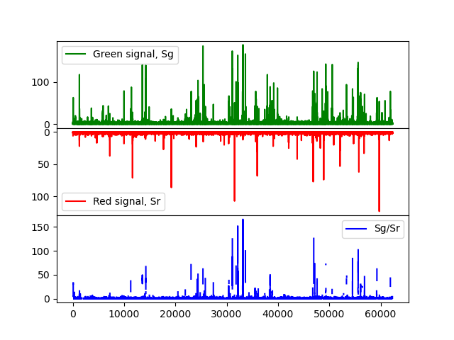
Above, for a donor and acceptor detection channel a histogram trace for is shown in green and red.

There are two options to compute intensity traces. Intensity traces can either be computed using the function tttrlib.compute_intensity_trace or using the method intensity_trace of a TTTR object.

tttr_object = tttrlib.TTTR('../../tttr-data/bh/bh_spc132.spc', 'SPC-130')
# option 1
tttr_object = tttrlib.compute_intensity_trace(
    data.macro_times,
    time_window_length=1.0, # this is one millisecond
    macro_time_resolution=data.get_header().macro_time_resolution / 1e6
)
# option 2
tttr_object = data.intensity_trace(
    time_window_length=1.0, # this is one millisecond
)

When the first option is used, a calibration for the macro time array needs to be provided. If the second option is used, the macro time calibration of the header information that was processes from the tttr file when the TTTR object was created is already considered. The time window length are in units of milli seconds.

/builds/skf/tttrlib/examples/single_molecule/plot_single_molecule_mcs.py:64: RuntimeWarning: divide by zero encountered in divide
  SgSr_ratio = (green_trace[:m] / red_trace[:m])
/builds/skf/tttrlib/examples/single_molecule/plot_single_molecule_mcs.py:64: RuntimeWarning: invalid value encountered in divide
  SgSr_ratio = (green_trace[:m] / red_trace[:m])
/builds/skf/tttrlib/examples/single_molecule/plot_single_molecule_mcs.py:65: RuntimeWarning: invalid value encountered in multiply
  SgSr_ratio[np.where((green_trace[:m] + red_trace[:m]) < 2)] *= 0

import matplotlib.pylab as p
import numpy as np

import tttrlib

data = tttrlib.TTTR('../../tttr-data/bh/bh_spc132.spc', 'SPC-130')
mt = data.get_macro_times()

green_indeces = data.get_selection_by_channel([0, 8])
red_indeces = data.get_selection_by_channel([1, 9])

fig, ax = p.subplots(3, 1, sharex=True, sharey=False)

p.setp(ax[0].get_xticklabels(), visible=False)
green_trace = tttrlib.compute_intensity_trace(
    mt[green_indeces],
    time_window_length=1.0e-3, # this is one millisecond
    macro_time_resolution=data.get_header().macro_time_resolution
)
red_trace = data[red_indeces].get_intensity_trace(
    time_window_length=1.0e-3
)
m = min(len(green_trace), len(red_trace))
SgSr_ratio = (green_trace[:m] / red_trace[:m])
SgSr_ratio[np.where((green_trace[:m] + red_trace[:m]) < 2)] *= 0

ax[0].plot(green_trace, 'g', label='Green signal, Sg')
ax[1].plot(red_trace, 'r', label='Red signal, Sr')
ax[1].invert_yaxis()
ax[0].legend()
ax[1].legend()
ax[2].plot(SgSr_ratio, 'b', label='Sg/Sr')
ax[2].legend()
p.subplots_adjust(
    left=None,
    bottom=None,
    right=None,
    top=None,
    wspace=None, hspace=0
)
p.show()
#