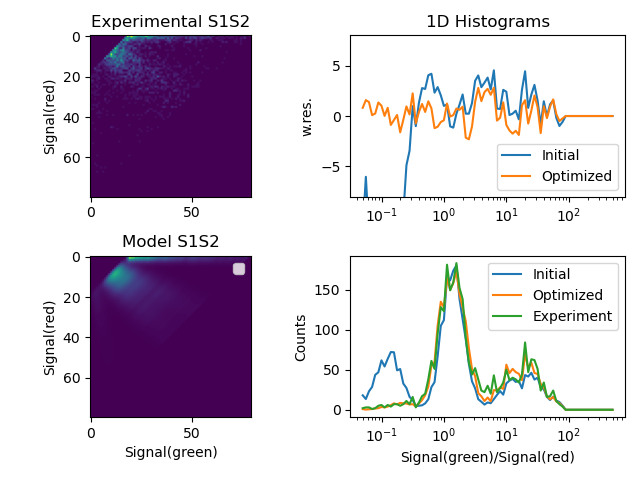
Photon distribution analysis - 2

Photon distribution analysis as described in https://pubs.acs.org/doi/abs/10.1021/jp057257

No artists with labels found to put in legend.  Note that artists whose label start with an underscore are ignored when legend() is called with no argument.

import glob
import numpy as np
import scipy.optimize
import pylab as plt
import tttrlib

"""
The experimental data is saved in separate files. The files are joined and the
resulting TTTR object is processed.
"""
# open a set of files and stack them in a single TTTR object
files = glob.glob('../../tttr-data/bh/bh_spc132_sm_dna/*.spc')
data = tttrlib.TTTR(files[0], 'SPC-130')
for d in files[1:]:
    data.append(tttrlib.TTTR(d, 'SPC-130'))

"""
As first step, the experimental counting histogram needs to be computed. For that,
the photon trace is split into time-windows (TWs) of a certain length (here 1 milli second).
The Photon Distribution Analysis (PDA) counting histogram is computed for two channels
(channel_1 and channel_2). The two channels are defined based on the routing channel
number. In the test data set, the routing channel numbers 0 and 8 correspond to the
green detection channels and the routing channel number 1 and 9 correspond to the
red detection channels.

The counting histogram is computed up to a maximum number of photons. Time windows
that have less photon counts than a certain number are discriminated from the counting
histogram.
"""
# Compute the experimental histograms
# # define what is PDA channel 1 and channel 2
channels_1 = [0, 8]  # 0, 8 are green channels
channels_2 = [1, 9]  # 1,9 are red channels
minimum_number_of_photons = 20
maximum_number_of_photons = 80
minimum_time_window_length = 1.0e-3

"""
The two dimensional counting histogram for the two channels is computed by the
static method ``tttrlib.Pda.compute_experimental_histograms`` that returns
additionally a one dimentional counting histogram of the photon number and an
array that contains pairs of start/stop indices of the TWs.
"""
s1s2_e, ps, tttr_indices = tttrlib.Pda.compute_experimental_histograms(
    tttr_data=data,
    channels_1=channels_1,
    channels_2=channels_2,
    maximum_number_of_photons=maximum_number_of_photons,
    minimum_number_of_photons=minimum_number_of_photons,
    minimum_time_window_length=minimum_time_window_length
)

"""
To compute a model counting histogram the minimum and maximum number of photons
need to be provided along with the probability of a certain total fluorescence P(F).
In this example P(F) is approximated by P(S). This approximation is invalid for
small number of photon counts. For a better estimation of P(F) see
https://pubs.acs.org/doi/abs/10.1021/jp072293p.
"""
# define a Pda object
kw_pda = {
    "hist2d_nmax": maximum_number_of_photons,
    "hist2d_nmin": minimum_number_of_photons,
    "pF": ps
}
pda = tttrlib.Pda(**kw_pda)

"""
The two dimensional counting histogram is usually marginalized to a one dimensional
representation. The 2D histogram of the counts are for instance marginalized to a
histogram over the ratio of the green and red photon counts or to a proximity
ratio histogram. The function that converts the 2D histogram to a 1D histogram is
assigned to the ``Pda`` object as a python function.
"""
# set a function to make a 1D histogram

# proximity ratio = Pr = Sg / (Sg + Sr)
# pda.histogram_function = lambda ch1, ch2: ch2 / max(1, (ch2 + ch1))

# ratio of green and red signal = Sg / Sr
pda.histogram_function = lambda ch1, ch2: ch1 / max(1, ch2)

"""
The background in the first and second channel controlled by corresponding
attributes.
"""
background_ch1 = 1.7
background_ch2 = 0.7
pda.background_ch1 = background_ch1
pda.background_ch2 = background_ch2

"""
The probabilities of detecting photons in the first channel with corresponding
amplitudes are passed as argument to a method that computes a 1D histogram in a
given range.
"""
amplitudes = [0.25, 0.25, 0.25, 0.25]
probabilities_ch1 = [0.0, 0.35, 0.45, 0.9]
kw_hist = {
    "x_max": 500.0,
    "x_min": 0.05,
    "log_x": True,
    "n_bins": 81,
    "n_min": 10
}
model_x, model_y = pda.get_1dhistogram(
    amplitudes=amplitudes,
    probabilities_ch1=probabilities_ch1,
    **kw_hist
)

"""
The corresponding experimental histogram is computed by passing the experimental
2D counting histogram as an argument.
"""
data_x, data_y = pda.get_1dhistogram(
    s1s2=s1s2_e.flatten(),
    **kw_hist
)
sd = np.sqrt(data_y)
np.place(sd, sd == 0, 10000000.0)
weighted_residuals = (data_y - model_y) / sd

"""
To optimize the parameters that determine the photon counting distribution we
define an objective function that quantifies the disagreement between the model
and the data and optimize the parameters of the objective function with
scipy.minimize.
"""


def chi2(
    x0: np.ndarray,
    y_data: np.ndarray,
    pda_object: tttrlib.Pda,
    n_species: int,
    kw_hist: dict
):
    amplitudes = x0[:n_species]
    probabilities = x0[n_species:n_species * 2]
    background_ch1 = x0[n_species * 2 + 0]
    background_ch2 = x0[n_species * 2 + 1]
    pda_object.background_ch1 = background_ch1
    pda_object.background_ch2 = background_ch2
    x_model, y_model = pda_object.get_1dhistogram(
        amplitudes=amplitudes,
        probabilities_ch1=probabilities,
        **kw_hist
    )
    wres = (y_data - y_model) / sd
    return np.sum(wres**2.0)


n_species = len(amplitudes)
x0 = np.array(amplitudes + probabilities_ch1 + [background_ch1, background_ch2])
bounds = [(0, np.inf)] * (2 * n_species) + [(0, 10), (0, 10)]
fit = scipy.optimize.minimize(
    fun=chi2,
    x0=x0,
    bounds=bounds,
    args=(data_y, pda, n_species, kw_hist),
)

"""
Plotting of the optimized histograms
"""
fitted_amplitudes = fit.x[:n_species]
fitted_probabilities_ch1 = fit.x[n_species:2*n_species]
fitted_background_ch1 = fit.x[n_species * 2 + 0]
fitted_background_ch2 = fit.x[n_species * 2 + 1]
pda.background_ch1 =fitted_background_ch1
pda.background_ch2 =fitted_background_ch2
model_fit_x, model_fit_y = pda.get_1dhistogram(
    amplitudes=fitted_amplitudes,
    probabilities_ch1=fitted_probabilities_ch1,
    **kw_hist
)
fit_wres = (data_y - model_fit_y) / sd

fig, ax = plt.subplots(nrows=2, ncols=2)
ax[0, 0].set_title('Experimental S1S2')
ax[0, 1].set_title('1D Histograms')
ax[1, 0].set_title('Model S1S2')
ax[0, 0].set_ylabel('Signal(red)')
ax[0, 1].set_ylabel('w.res.')
ax[1, 1].set_xlabel('Signal(green)/Signal(red)')
ax[1, 1].set_ylabel('Counts')
ax[1, 0].set_xlabel('Signal(green)')
ax[1, 0].set_ylabel('Signal(red)')
ax[0, 0].imshow(s1s2_e[1:, 1:])
ax[1, 0].imshow(pda.s1s2[1:, 1:])
ax[1, 0].legend()

fit_wres = np.nan_to_num(fit_wres, posinf=0, neginf=0)
y_model_initial = np.nan_to_num(model_y, posinf=0, neginf=0)
ax[0, 1].set_ylim(-8, 8)
if kw_hist['log_x']:
    ax[0, 1].semilogx(data_x, weighted_residuals, label="Initial")
    ax[0, 1].semilogx(data_x, fit_wres, label="Optimized")
    ax[1, 1].semilogx(model_x, y_model_initial, label="Initial")
    ax[1, 1].semilogx(model_fit_x, model_fit_y, label="Optimized")
    ax[1, 1].semilogx(data_x, data_y, label="Experiment")
else:
    ax[0, 1].plot(data_x, weighted_residuals, label="Initial")
    ax[0, 1].plot(data_x, fit_wres, label="Optimized")
    ax[1, 1].plot(model_x, y_model_initial, label="Initial")
    ax[1, 1].plot(model_fit_x, model_fit_y, label="Optimized")
    ax[1, 1].plot(data_x, data_y, label="Experiment")
ax[1, 1].legend()
ax[0, 1].legend()
plt.tight_layout()
plt.show()