Accessible volume decorator

IMP particles can be decorated with accessible volume (AV) decorators to compute the sterically allowed volume of a label around its attachment site, i.e., the decorated IMP particle.

The AV decorator uses the Dijkstra’s algorithm to compute all path from the attachment site to a set of grid points around the attachment site. The AV decorator uses the IMP.bff.PathMap class for computing the AV. The occupied volume of leaves in a molecular hierarchy serve as obstacles in the path search.

import pathlib
import numpy as np
import pylab as plt

import IMP
import IMP.core
import IMP.atom
import IMP.em
import IMP.bff

Setup Model

m = IMP.Model()
pdb_fn = pathlib.Path(IMP.bff.get_example_path('structure')) / "T4L/3GUN.pdb"
hier = IMP.atom.read_pdb(str(pdb_fn), m)

Decorate particle

Any particle can be decorated by AVs. The location of the AV particle is changed by AV calculation to the mean position of the AV. Thus, better create a new particle that will be decorated with an AV.

av_p = IMP.Particle(m)

An AV has a source, i.e., the labeling site and a set of parameters that determine the shape of the AV. We select

residue_index = 132
atom_name = "CB"
sel = IMP.atom.Selection(hier)
sel.set_atom_type(IMP.atom.AtomType(atom_name))
sel.set_residue_index(residue_index)
source = sel.get_selected_particles()[0]
av_parameter = {
    "linker_length": 20.0,
    "radii": (3.5, 0.0, 0.0),
    "linker_width": 0.5,
    "allowed_sphere_radius": 2.0,
    "contact_volume_thickness": 0.0,
    "contact_volume_trapped_fraction": -1,
    "simulation_grid_resolution": 0.5
}
IMP.bff.AV.do_setup_particle(m, av_p, source, **av_parameter)
av1 = IMP.bff.AV(m, av_p)

The coordinates of an AV are the mean AV the density map. Thus, the position of the AV changes when the AV is resampled.

av_xyz = IMP.core.XYZ(av1)
# av_mp == (0,0,0)
av1.resample()  # Updates the AV
# av_xyz == (-1.46132, -25.366, -6.04022)

Access AV features

AV decorated particles use PathMaps to sample the accessible volume. Thus, features of the AV are accesses trough PathMap. The features can be written to density maps (see: PathMapTile). PathMaps derive from IMP EM density maps and sampled obstacles can be written to density files using standard IMP methods.

av_map = av1.get_map()
bounds = 0.01, 20
# write to map
#IMP.em.write_map(av_map, "OBSTACLES.mrc")

Features of a IMP.bff.PathMap are identified by the following constants

pm_features = [
    IMP.bff.PM_TILE_PENALTY,             # Penality of visiting a tile
    IMP.bff.PM_TILE_COST,                # Cost of a path to the tile
    IMP.bff.PM_TILE_DENSITY,             # Density of tile
    IMP.bff.PM_TILE_COST_DENSITY,        # Cost * Density of tile
    IMP.bff.PM_TILE_PATH_LENGTH,         # Path length to tile (cost * grid spacing)
    IMP.bff.PM_TILE_PATH_LENGTH_DENSITY, # Path length to tile * density
    IMP.bff.PM_TILE_FEATURE,             # Additional feature of tile (accessed by name)
    IMP.bff.PM_TILE_ACCESSIBLE_DENSITY,  # Density of tiles with path length in bounds
    IMP.bff.PM_TILE_ACCESSIBLE_FEATURE   # Feature of tile with path length in bounds
]

These features can be written to density maps

# IMP.bff.write_path_map(
#     av_map, "BFF_TILE_PENALTY.mrc",
#     IMP.bff.PM_TILE_PENALTY,
#     (0, 1)
# )

# PM_TILE_PATH_LENGTH_WEIGHT : filter by path length and write tile weight
# IMP.bff.write_path_map(
#     av_map, "PM_TILE_PATH_LENGTH.mrc",
#     IMP.bff.PM_TILE_PATH_LENGTH,
#     bounds
# )

# IMP.bff.write_path_map(
#     av_map, "PM_TILE_PATH_LENGTH_DENSITY_132.mrc",
#     IMP.bff.PM_TILE_PATH_LENGTH_DENSITY,
#     bounds
# )

# IMP.bff.write_path_map(
#     av_map, "PM_TILE_ACCESSIBLE_DENSITY.mrc",
#     IMP.bff.PM_TILE_ACCESSIBLE_DENSITY,
#     bounds
# )

Measure AV/AV-distance

residue_index = 55
sel = IMP.atom.Selection(hier)
sel.set_atom_type(IMP.atom.AtomType("CB"))
sel.set_residue_index(residue_index)
p = sel.get_selected_particles()[0]
av_p2 = IMP.Particle(m)
IMP.bff.AV.do_setup_particle(m, av_p2, p, **av_parameter)
av2 = IMP.bff.AV(av_p2)
v = IMP.bff.av_distance(av1, av2)
print(v)

55.642224549950214

Distance types

distance_types = [
    IMP.bff.DYE_PAIR_DISTANCE_E,             # Mean FRET averaged distance R_E
    IMP.bff.DYE_PAIR_DISTANCE_MEAN,          # Mean distance <R_DA>
    IMP.bff.DYE_PAIR_DISTANCE_MP,            # Distance between AV mean positions
    IMP.bff.DYE_PAIR_EFFICIENCY,             # Mean FRET efficiency
    IMP.bff.DYE_PAIR_DISTANCE_DISTRIBUTION,  # (reserved for Distance distributions)
    IMP.bff.DYE_PAIR_XYZ_DISTANCE            # Distance between XYZ of dye particles
]

forster_radius = 52.0 # Optional (default 52.0)
n_samples = 20000     # Optional (default 10000)
fret_efficiency = IMP.bff.av_distance(
    av1, av2,
    forster_radius=forster_radius,
    distance_type=IMP.bff.DYE_PAIR_EFFICIENCY,
    n_samples=n_samples
)
distance_fret = IMP.bff.av_distance(
    av1, av2,
    forster_radius,
    IMP.bff.DYE_PAIR_DISTANCE_E,
    n_samples
)
mean_inter_dye_distance = IMP.bff.av_distance(av1, av2, distance_type=IMP.bff.DYE_PAIR_DISTANCE_MEAN)
print("Mean FRET efficiency   : {:.2f}".format(fret_efficiency))
print("Distance FRET          : {:.1f}".format(distance_fret))
print("Mean inter-dye distance: {:.1f}".format(mean_inter_dye_distance))
print("Distance mean position : {:.1f}".format(IMP.bff.av_distance(av1, av2, IMP.bff.DYE_PAIR_DISTANCE_MP)))

Mean FRET efficiency   : 0.43
Distance FRET          : 54.5
Mean inter-dye distance: 55.4
Distance mean position : 55.4

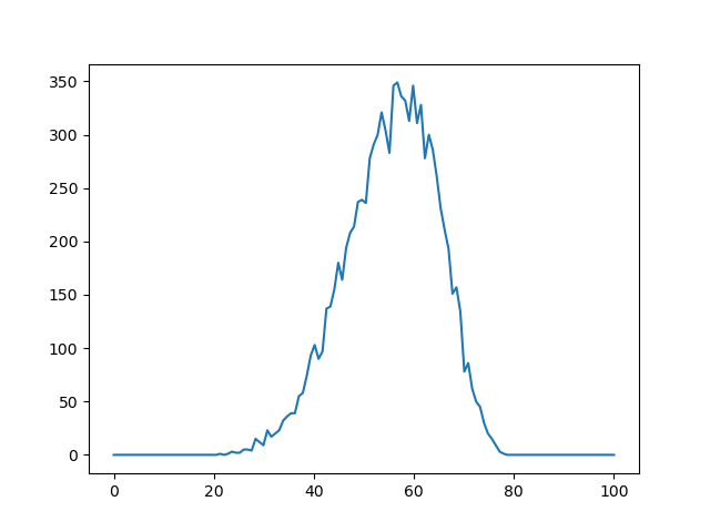
Distance distribution between two AVs

rda_start, rda_stop, n_bins = 0, 100, 128
n_samples = 10000
rda = np.linspace(rda_start, rda_stop, n_bins)
p_rda = IMP.bff.av_distance_distribution(av1, av2, rda, n_samples=n_samples)
plt.plot(rda, p_rda)
plt.show()