Scoring of structures

This examples illustrates how to use IMP.bff.AVNetworkRestraint for scoring structures in a trajectory.

import json
import tqdm
import pylab as plt

import RMF
import IMP
import IMP.rmf
import IMP.atom
import IMP.bff

Load an RMF file and create a hierarchy

print("Creating IMP Model")
m = IMP.Model()
rmf_fn = IMP.bff.get_example_path("structure/T4L/t4l_docking.rmf3")

print("Loading RMF")
frame_index = 0
f = RMF.open_rmf_file_read_only(rmf_fn)
hier = IMP.rmf.create_hierarchies(f, m)[frame_index]
IMP.rmf.load_frame(f, RMF.FrameID(frame_index))

Creating IMP Model
Loading RMF

Load fps.json file and create restraint for scoring

print("Creating FRET restraint")
fps_json_path = IMP.bff.get_example_path("structure/T4L/fret.fps.json")
with open(fps_json_path) as fp:
    fps_json = json.load(fp)
score_set_c1 = "chi2_C1_33p"
fret_restraint = IMP.bff.AVNetworkRestraint(
    hier, fps_json_path,
    score_set=score_set_c1
)
v = fret_restraint.unprotected_evaluate(None)

Creating FRET restraint

Score each frame in the RMF file and plot score

print("Scoring frames")
scores = list()
for frame in tqdm.tqdm(f.get_root_frames()):
    IMP.rmf.load_frame(f, frame)
    v = fret_restraint.unprotected_evaluate(None)
    scores.append(v)

Scoring frames

  0%|          | 0/100 [00:00<?, ?it/s]
  2%|▏         | 2/100 [00:00<00:07, 13.75it/s]
  4%|▍         | 4/100 [00:00<00:07, 13.22it/s]
  6%|▌         | 6/100 [00:00<00:07, 13.22it/s]
  8%|▊         | 8/100 [00:00<00:06, 13.63it/s]
 10%|█         | 10/100 [00:00<00:06, 13.84it/s]
 12%|█▏        | 12/100 [00:00<00:06, 14.01it/s]
 14%|█▍        | 14/100 [00:01<00:06, 14.14it/s]
 16%|█▌        | 16/100 [00:01<00:05, 14.21it/s]
 18%|█▊        | 18/100 [00:01<00:05, 14.08it/s]
 20%|██        | 20/100 [00:01<00:05, 14.09it/s]
 22%|██▏       | 22/100 [00:01<00:05, 13.76it/s]
 24%|██▍       | 24/100 [00:01<00:05, 13.70it/s]
 26%|██▌       | 26/100 [00:01<00:05, 13.43it/s]
 28%|██▊       | 28/100 [00:02<00:05, 13.61it/s]
 30%|███       | 30/100 [00:02<00:05, 13.83it/s]
 32%|███▏      | 32/100 [00:02<00:04, 14.08it/s]
 34%|███▍      | 34/100 [00:02<00:04, 13.94it/s]
 36%|███▌      | 36/100 [00:02<00:04, 14.13it/s]
 38%|███▊      | 38/100 [00:02<00:04, 14.25it/s]
 40%|████      | 40/100 [00:02<00:04, 14.25it/s]
 42%|████▏     | 42/100 [00:03<00:04, 14.29it/s]
 44%|████▍     | 44/100 [00:03<00:03, 14.38it/s]
 46%|████▌     | 46/100 [00:03<00:03, 14.51it/s]
 48%|████▊     | 48/100 [00:03<00:03, 14.49it/s]
 50%|█████     | 50/100 [00:03<00:03, 14.65it/s]
 52%|█████▏    | 52/100 [00:03<00:03, 14.69it/s]
 54%|█████▍    | 54/100 [00:03<00:03, 14.63it/s]
 56%|█████▌    | 56/100 [00:03<00:02, 14.81it/s]
 58%|█████▊    | 58/100 [00:04<00:02, 14.94it/s]
 60%|██████    | 60/100 [00:04<00:02, 14.96it/s]
 62%|██████▏   | 62/100 [00:04<00:02, 14.65it/s]
 64%|██████▍   | 64/100 [00:04<00:02, 14.68it/s]
 66%|██████▌   | 66/100 [00:04<00:02, 14.86it/s]
 68%|██████▊   | 68/100 [00:04<00:02, 14.55it/s]
 70%|███████   | 70/100 [00:04<00:02, 14.59it/s]
 72%|███████▏  | 72/100 [00:05<00:01, 14.66it/s]
 74%|███████▍  | 74/100 [00:05<00:01, 14.79it/s]
 76%|███████▌  | 76/100 [00:05<00:01, 14.86it/s]
 78%|███████▊  | 78/100 [00:05<00:01, 14.86it/s]
 80%|████████  | 80/100 [00:05<00:01, 14.91it/s]
 82%|████████▏ | 82/100 [00:05<00:01, 14.95it/s]
 84%|████████▍ | 84/100 [00:05<00:01, 14.94it/s]
 86%|████████▌ | 86/100 [00:05<00:00, 14.97it/s]
 88%|████████▊ | 88/100 [00:06<00:00, 15.00it/s]
 90%|█████████ | 90/100 [00:06<00:00, 14.99it/s]
 92%|█████████▏| 92/100 [00:06<00:00, 14.97it/s]
 94%|█████████▍| 94/100 [00:06<00:00, 14.97it/s]
 96%|█████████▌| 96/100 [00:06<00:00, 15.14it/s]
 98%|█████████▊| 98/100 [00:06<00:00, 15.32it/s]
100%|██████████| 100/100 [00:06<00:00, 15.35it/s]
100%|██████████| 100/100 [00:06<00:00, 14.49it/s]

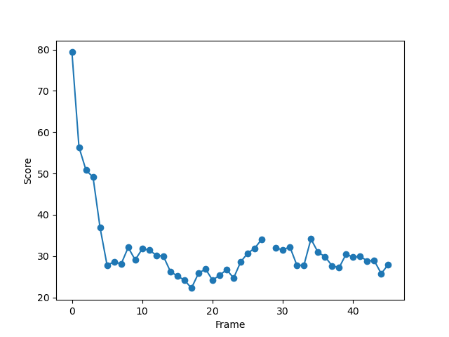
Plot score for each frame

plt.plot(scores, "o-")
plt.xlabel("Frame")
plt.ylabel("Score")
plt.show()