Orientation factor

Compute the probability of distance distributions for an experimental steady state donor and acceptor anisotropies.

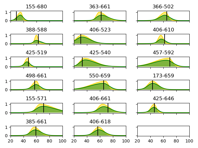
155-680
exp_mean: 34.403080708441536 29.2 4.97524512776874
363-661
exp_mean: 65.43651035746336 62.0 9.761023084699954
366-502
exp_mean: 61.44798310309122 65.4 8.506476812570064
388-588
exp_mean: 61.24354756859989 63.2 6.092983866995865
406-523
exp_mean: 35.95518607205667 30.4 10.886374749306476
406-610
exp_mean: 57.2128011004459 62.2 6.436227506895058
425-519
exp_mean: 45.18657151924009 47.6 4.984525757756681
425-540
exp_mean: 44.226926077433745 33.2 12.762766598147058
457-592
exp_mean: 56.32112758588779 70.1 15.112524182270327
498-661
exp_mean: 58.7713175694632 57.4 7.1600777615081865
550-659
exp_mean: 56.24407498741824 65.8 14.601376425919101
173-659
exp_mean: 45.17511881019857 43.5 8.791703363295433
155-571
exp_mean: 77.8743308713932 71.1 14.900485345976827
406-661
exp_mean: 67.96645190082295 72.4 10.431468244777335
425-646
exp_mean: 45.37992353849717 46.5 5.870371779101921
385-661
exp_mean: 59.76550281374226 59.3 8.77752558483804
406-618
exp_mean: 59.184372374597885 56.9 8.954501380333214

import numpy as np
import numba as nb
import scipy.stats

import pylab as plt
from matplotlib.ticker import (MultipleLocator, AutoMinorLocator)
import IMP.bff.spectroscopy.kappa2
from IMP.bff.spectroscopy.kappa2 import s2delta, kappasq_all_delta


@nb.njit
def normal_dist(x, loc, scale):
    prob_density = (np.pi*scale) * np.exp(-0.5*((x-loc)/scale)**2)
    return prob_density


@nb.njit
def normal_dist_np(x, loc, scale_neg, scale_pos):
    prob_density = np.empty_like(x)
    for i, xi in enumerate(x):
        if xi < loc:
            prob_density[i] = np.exp(-0.5*((xi-loc)/scale_neg)**2)
        else:
            prob_density[i] = np.exp(-0.5*((xi-loc)/scale_pos)**2)
    return prob_density


def mean_sd(axis, value) -> float:
    s = np.sum(value)
    v = np.dot(axis, value)
    v /= s
    v2 = np.dot(axis**2.0, value)
    v2 /= s
    return v, v2 - v**2.0


@nb.jit
def RDA_coupler(
        RDA_ax,
        Rapp_ax, Rapp_pdf,
        k2_ax, k2_pdf,
        scale=0.01
) -> np.ndarray:
    RDA_pdf = np.zeros_like(RDA_ax, dtype=np.float64)
    for i, RDA in enumerate(RDA_ax):
        for pRapp, Rapp in zip(Rapp_pdf, Rapp_ax):
            for pk2, k2 in zip(k2_pdf, k2_ax):
                v = (3./2. * k2)**(1./6) * Rapp
                delta = RDA - v
                # Use norm dist instead of delta
                # delta need equality which can be hard to
                # get in discrete space
                pr = normal_dist(
                    delta,
                    0.0,
                    scale
                )
                RDA_pdf[i] += pr * pRapp * pk2
    return RDA_pdf


def k2_call(
        **kwargs
):
    sD2 = kwargs['sD2']
    sA2 = kwargs['sA2']
    step = kwargs['step']
    n_bins = kwargs['n_bins']
    r_0 = kwargs['r_0']
    _, delta = s2delta(
        s2_donor=sD2,
        s2_acceptor=sA2,
        r_inf_AD=kwargs.get(r_ADinf, 0.0001),
        r_0=r_0
    )
    return kappasq_all_delta(
        delta = delta,
        sD2 = sD2,
        sA2 = sA2,
        step = step,
        n_bins = n_bins
    )


n_axis = 256
r_min = 10
r_max = 120
k2_min, k2_max = 0.1, 4.0

names = ["155-680", "363-661", "366-502", "388-588", "406-523", "406-610", "425-519", "425-540", "457-592", "498-661", "550-659", "173-659", "155-571", "406-661", "425-646", "385-661", "406-618"]
r_inf_DDs = [0.246, 0.298, 0.23, 0.231, 0.293, 0.279, 0.137, 0.137, 0.137, 0.237, 0.201, 0.192, 0.223, 0.193, 0.195, 0.195, 0.193]
r_inf_AAs = [0.165, 0.241, 0.214, 0.231, 0.221, 0.178, 0.169, 0.214, 0.206, 0.156, 0.177, 0.217, 0.212, 0.145, 0.209, 0.227, 0.186]
r_ADinfs = [0.01, 0.026, 0.041, 0.049, 0.012, 0.02, 0.105, 0.0561, 0.091, 0.112, 0.018, 0.007, 0.02, 0.019, 0.05, 0.05, 0.017]

distance_sets = {
    'R1': {
        'Rapp_ms': [78.2, 81.8, 32.9, 60.0, 44.2, 38.9, 34.0, 57.4, 52.5, 43.7, 56.8, 68.5, 46.4, 37.6, 74.7, 75.5, 43.4],
        'RDA_ref': [87.0, 78.0, 23.5, 65.0, 43.7, 42.3, 39.0, 57.5, 65.6, 53.2, 64.4, 74.9, 51.8, 36.2, 77.0, 77.0, 52.9],
        'Rapp_sd': [(9.1, 6.2), (27.0, 5.2), (7.2, 7.2), (2.5, 2.5), (4.1, 1.9), (3.4, 4.2), (6.2, 14.1), (3.0, 2.1), (7.6, 12.6), (3.6, 5.0), (6.4, 11.9), (5.9, 10.4), (5.9, 3.0), (3.1, 3.4), (8.8, 9.0), (8.2, 9.3), (4.9, 5.4)]
    },
    'R2': {
        'Rapp_ms': [35.8, 59.0, 63.3, 60.0, 31.9, 56.3, 46.4, 36.0, 68.4, 60.0, 68.8, 43.3, 65.6, 64.0, 45.9, 56.5, 58.0],
        'RDA_ref': [29.2, 62.0, 65.4, 63.2, 30.4, 62.2, 47.6, 33.2, 70.1, 57.4, 65.8, 43.5, 71.1, 72.4, 46.5, 59.3, 56.9],
        'Rapp_sd': [(5.0, 2.5), (4.3, 10.1), (8.1, 4.3), (2.5, 2.5), (8.2, 12.0), (4.0, 3.6), (3.9, 2.1), (6.6, 16.5), (21.6, 5.6), (6.1, 3.4), (21.2, 4.2), (6.9, 8.4), (5.9, 20.4), (6.3, 10.4), (4.9, 3.4), (5.3, 8.2), (6.9, 7.4)]
    }
}
exp_means = {}

# Plot here only the first distance set
for ds in list(distance_sets.keys())[1:]:
    Rapp_ms = distance_sets[ds]['Rapp_ms']
    Rapp_m_refs = distance_sets[ds]['RDA_ref']
    Rapp_sds = distance_sets[ds]['Rapp_sd']

    angle_step_size = 0.15
    r0 = 0.38
    ncols = 3
    nrows = 6
    fig, axs = plt.subplots(nrows, ncols, sharex=True, sharey=True)
    expm = list()
    exp_means[ds] = expm

    for i in range(len(names)):
        name = names[i]
        print(name)
        row, col = 0, 0
        ax = axs.flatten()[i]
        # Make a plot with major ticks that are multiples of 20 and minor ticks that
        # are multiples of 5.  Label major ticks with '.0f' formatting but don't label
        # minor ticks.  The string is used directly, the `StrMethodFormatter` is
        # created automatically.
        ax.xaxis.set_major_locator(MultipleLocator(20))
        ax.set_xlim(left=20, right=100)
        ax.set_title(name)
        r_inf_DD = r_inf_DDs[i]
        r_inf_AA = r_inf_AAs[i]
        r_ADinf = r_ADinfs[i]
        Rapp_m = Rapp_ms[i]
        Rapp_m_ref = Rapp_m_refs[i]
        Rapp_sd = Rapp_sds[i]

        k2_kw = {
            'step': angle_step_size,
            'n_bins': n_axis,
            'sD2': -np.sqrt(r_inf_DD / r0),
            'sA2': np.sqrt(r_inf_AA / r0),
            'r_ADinf': r_ADinf,
            'r_0': r0
        }

        k2_axis, k2_mean_histogram, k2 = k2_call(**k2_kw)
        k2_pdf_wic = k2_mean_histogram
        # use norm dist for Rapp
        k2_ax = k2_axis[1:]
        _, k2_sd = mean_sd(k2_ax, k2_pdf_wic)

        # Use norm distirbution with width ovls
        # instead of delta function (numeric stability)
        ovls = (r_max - r_min) / (2 * n_axis)

        Rapp_ax = np.linspace(r_min, r_max, n_axis)
        RDA_ax = np.linspace(r_min, r_max, n_axis)
        Rapp_pdf = normal_dist_np(Rapp_ax, Rapp_m, *Rapp_sd)

        k2_pdf_wic /= sum(k2_pdf_wic)
        RDA_pdf_wic_k2 = RDA_coupler(
            RDA_ax,
            Rapp_ax, Rapp_pdf,
            k2_ax, k2_pdf_wic,
            scale=ovls
        )

        k2_wic = k2_pdf_wic

        exp_mean = np.dot(RDA_pdf_wic_k2, RDA_ax) / np.sum(RDA_pdf_wic_k2)
        ref_mean = Rapp_m_ref
        exp_mean2 = np.dot(RDA_pdf_wic_k2, RDA_ax**2) / np.sum(RDA_pdf_wic_k2)
        exp_sd = np.sqrt(exp_mean2 - exp_mean**2.0)
        expm.append([exp_mean, ref_mean, exp_sd])
        print('exp_mean:', exp_mean, ref_mean, exp_sd)

        ymax = max(Rapp_pdf)*1.1
        ax.plot(Rapp_ax, Rapp_pdf, label='Rapp', color='gold')
        ax.fill_between(Rapp_ax, 0.0, Rapp_pdf, facecolor='gold', alpha=0.5)
        ax.plot(Rapp_ax, RDA_pdf_wic_k2, label='RDA_pdf_wic_k2', color='green')
        ax.fill_between(Rapp_ax, 0.0, RDA_pdf_wic_k2, facecolor='green', alpha=0.5)
        ax.vlines(x=Rapp_m_ref, ymin=0.0, ymax=ymax, linestyles='solid', colors=['black'])

    plt.tight_layout()
    fname = ds + '.png'
    # plt.savefig(path + fname, dpi=300)
    fig.show()